By Dexter Davis - Research Technician for Dr. Shawn Arellano

This Markdown file summarizes the larval data collected with the SyPRID collector on the AUV Sentry during the 2020 EN658 and 2021 TN391 SALT project cruises. This is part of the Seep Animal Larval Transport (SALT) project, NSF Award #1851286.

This markdown file will summarize the data by site as well as by depth classification. Depth classification are as follows: Demersal - 5 meters above bottom, Low Water Column - 80 meters above bottom, Thermocline - depths varied between sites, Mid Water Column - a midway depth between the thermocline and demersal depths.

Data Entry and Subsetting

#install.packages("ggplot2")
library(PNWColors)
library(ggplot2)
library(readxl)
library(knitr)
library(RColorBrewer)
library(gplots)
library(qrcode)
library(vegan)
library(reshape2)
library(ggdendro)
library(plyr)

setwd("C:/Users/davis/OneDrive/Desktop/SPMC Work/Morphotype Consensus")

## Every Dive from Both Cruises
Dive <- read_xlsx("SALT_Larval_Consensus_Final_COPY.xlsx", sheet = "Larval Total Counts")
Dive <- Dive[-c(43),]
Dive <- subset(Dive[-c(7:153)])

## Number of Dives per Site and Depth Classification
Dives <- read_xlsx("SALT_Larval_Consensus_Final_COPY.xlsx", sheet = "Number of Dives")
SiteD <- subset(Dives[-c(1:3)])
colnames(SiteD) <- c("Site","Number of Dives","Average Flow Rate (L/min)")
DepthD <-subset(Dives[-c(4:6)])
DepthD <- na.omit(DepthD)
colnames(DepthD) <- c("Depth Classification","Number of Dives","Average Flow Rate (L/min)")


## Average Volume Collected, Larvae Collected, Larval Density per Site and Depth Classification
Avgs <- read_xlsx("SALT_Larval_Consensus_Final_COPY.xlsx", sheet = "Averages")
SiteAvg <- subset(Avgs[-c(8:15)])
SVol <- subset(SiteAvg[-c(4:7)])
SLar <- subset(SiteAvg[-c(2:3,6:7)])
SDen <- subset(SiteAvg[-c(2:5)])
SDen <- subset(SDen, SDen$Site != "Florida Keys")

DepthAvg <- subset(Avgs[-c(1:8)])
DepthAvg <- na.omit(DepthAvg) 
DVol <- subset(DepthAvg[-c(4:7)])
DLar <- subset(DepthAvg[-c(2:3,6:7)])
DDen <- subset(DepthAvg[-c(2:5)])

## Site data untouched - has each site and depth classifications within
Site <- read_xlsx("SALT_Larval_Consensus_Final_COPY.xlsx", sheet = "Larval Density by Site an Depth")
BaltimoreCanyon <- subset(Site,Site$`Sample Site`=="Baltimore Canyon")
BlakeRidge <- subset(Site,Site$`Sample Site`=="Blake Ridge") 
BrinePool <- subset(Site,Site$`Sample Site`=="Brine Pool")
BushHill <- subset(Site,Site$`Sample Site`=="Bush Hill")
Chincoteague <- subset(Site,Site$`Sample Site`=="Chincoteague")
FloridaEscarpment <- subset(Site,Site$`Sample Site`=="Florida Escarpment")
GC234 <- subset(Site,Site$`Sample Site`=="Green Canyon 234")
MississippiCanyon <- subset(Site,Site$`Sample Site`=="Mississippi Canyon")

## Larval Type Code Guide
Guide <- read_xlsx("SALT_Larval_Consensus_Final_COPY.xlsx", sheet ="Larval Type Guide")

## Larval Type Presence by Depth
LarvDepth <- read_xlsx("SALT_Larval_Consensus_Final_COPY.xlsx", sheet ="Larval Type by Depth")

LDDem <- subset(LarvDepth,LarvDepth$`Depth Classification`=="Demersal")
LDDem <- subset(LDDem[-c(1)])
LDMWC <- subset(LarvDepth,LarvDepth$`Depth Classification`=="Mid Water Column")
LDMWC <- subset(LDMWC[-c(1)])
LDTherm <- subset(LarvDepth,LarvDepth$`Depth Classification`=="Thermocline")
LDTherm <- subset(LDTherm[-c(1)])

Summary of Dives from EN658 and TN391

~~~~~~~~~~~~~~~~~~~~~~~~~~~~~~~~~~~~~~~~~~~~~~

Cruise	Site	Dive # / Code	Method	Depth (meters, mab= meters above bottom)	Depth Classification
EN658	Baltimore Canyon	HN0	Hand Net	0	Surface
EN658	Baltimore Canyon	HN200	Hand Net	0-200	Upper Water Column
EN658	Baltimore Canyon	HN200B	Hand Net	0-200	Upper Water Column
EN658	Blake Ridge	S569P	Sentry	5mab	Demersal
EN658	Blake Ridge	S569S	Sentry	80mab	Lower Water Column
EN658	Blake Ridge	S570S	Sentry	5-195mab	Lower Water Column
EN658	Blake Ridge	BR200	Hand Net	0-200	Upper Water Column
EN658	Blake Ridge	BR200B	Hand Net	0-200	Upper Water Column
EN658	Brine Pool	S572S	Sentry	5mab	Demersal
EN658	Brine Pool	S572P	Sentry	80mab	Mid Water Column
EN658	Brine Pool	BP200	Hand Net	0-200	Upper Water Column
EN658	Brine Pool	BP200B	Hand Net	0-200	Upper Water Column
EN658	Bush Hill	BH200B	Hand Net	0-200	Upper Water Column
EN658	Bush Hill	BH200C	Hand Net	0-200	Upper Water Column
EN658	Florida Keys	FK200	Hand Net	0-200	Upper Water Column
EN658	Florida Keys	FK200B	Hand Net	0-200	Upper Water Column
EN658	Mississippi Canyon	MC200	Hand Net	0-200	Upper Water Column
EN658	Mississippi Canyon	MC200B	Hand Net	0-200	Upper Water Column
TN391	Baltimore Canyon	S583P	Sentry	10mab (420)	Demersal
TN391	Baltimore Canyon	S584P	Sentry	5mab (425)	Demersal
TN391	Baltimore Canyon	S585P	Sentry	5mab (380)	Demersal
TN391	Baltimore Canyon	S584S	Sentry	300	Mid Water Column
TN391	Baltimore Canyon	S583S	Sentry	200	Thermocline
TN391	Blake Ridge	S587P	Sentry	5mab (2160)	Demersal
TN391	Blake Ridge	S588P	Sentry	5mab (2163)	Demersal
TN391	Blake Ridge	S587S	Sentry	200	Thermocline
TN391	Blake Ridge	S588S	Sentry	200	Thermocline
TN391	Brine Pool	S592P	Sentry	5mab (500)	Demersal
TN391	Brine Pool	S593P	Sentry	5mab	Demersal
TN391	Brine Pool	S592S	Sentry	300	Mid Water Column
TN391	Brine Pool	S593S	Sentry	200	Thermocline
TN391	Bush Hill	S594P	Sentry	5mab	Demersal
TN391	Bush Hill	S594S	Sentry	300	Mid Water Column
TN391	Chincoteague	S586P	Sentry	5mab (995)	Demersal
TN391	Florida Escarpment	S589P	Sentry	5mab (3300)	Demersal
TN391	Florida Escarpment	S590S	Sentry	1700	Mid Water Column
TN391	Florida Escarpment	S589S	Sentry	200	Thermocline
TN391	Florida Keys	HN200FK	Hand Net	200	Surface
TN391	Green Canyon 234	S591P	Sentry	5mab (500)	Demersal
TN391	Green Canyon 234	S591S	Sentry	300	Mid Water Column
TN391	Mississippi Canyon	S595P	Sentry	5mab	Demersal
TN391	Mississippi Canyon	S595S	Sentry	600	Mid Water Column

The rest of this markdown file and data analysis will focus only on the TN391 Sentry dives (this exludes Florida Keys Hand Net) and the EN658 Brine Pool Sentry dives (S572S/S572P). Brine Pool was the only EN658 site that had comparable depths to TN391, and Sentry did not malfunction (EN658 Blake Ridge).

Sentry Performance

Summary Tables of Number of Dives

~~~~~~~~~~~~~~~~~~~~~~~~~~~~~~~~~~~~~~~~~~~~~~

Number of Dives per Site
Site	Number of Dives	Average Flow Rate (L/min)
Baltimore Canyon	5	11521.929
Blake Ridge	4	10900.721
Brine Pool	5	12619.784
Bush Hill	2	9334.150
Chincoteague	1	11569.161
Florida Escarpment	3	12849.621
Green Canyon 234	2	11067.122
Mississippi Canyon	2	9261.488

Flow Rate Range: 9,261-12,850 Liters/min

Number of Dives per Depth Classification
Depth Classification	Number of Dives	Average Flow Rate (L/min)
Demersal	13	8673.924
Mid Water Column	6	10489.760
Thermocline	5	19611.084

Flow Rate Range: 8,674-19,611 Liters/min

Statistics Between Sites and Depth Classifications

~~~~~~~~~~~~~~~~~~~~~~~~~~~~~~~~~~~~~~~~~~~~~~

Sites

Volume Sampled

#SVol
my_title <- "Average Volume of Water Collected by SyPRID by Site"
ggplot(SVol, aes(x=SVol$Site, y=SVol$`Avg Volume Sampled`))+geom_bar(fill="deepskyblue3",stat="identity",position=position_dodge(),width = 0.9)+labs(title =my_title, x="Site", y="Average Volume Collected (L)")+theme(plot.title = element_text(hjust=0.5), axis.text.x=element_text(angle = 45, vjust = 1, hjust=1))+geom_errorbar(aes(ymin=SVol$`Avg Volume Sampled`- SVol$`Volume STDev...3`, ymax=SVol$`Avg Volume Sampled`+ SVol$`Volume STDev...3`), width=.2,position=position_dodge(.9))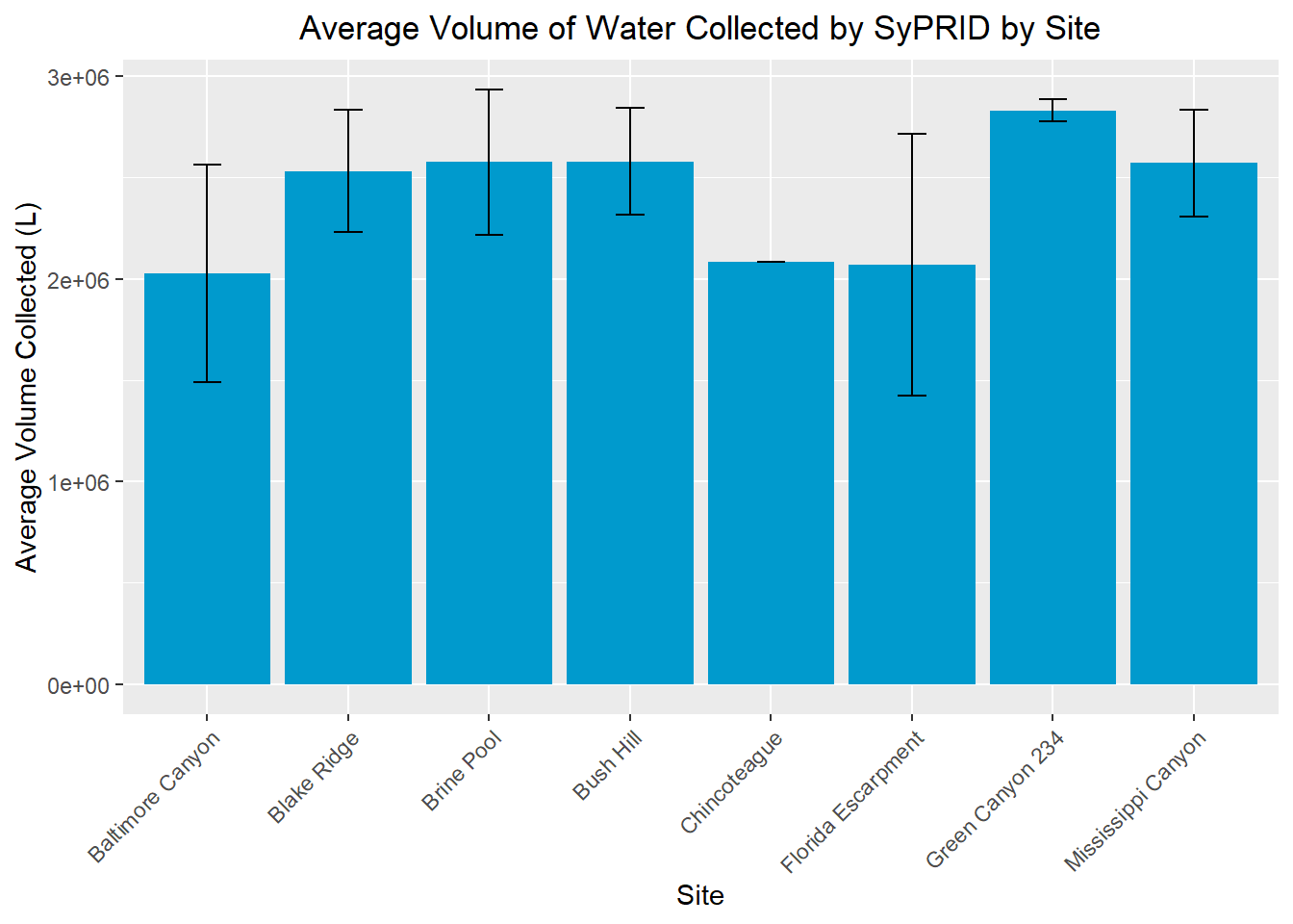

Larvae Collected

#SLAr
my_title <- "Average Number of Larvae Collected by SyPRID by Site"
ggplot(SLar, aes(x=SLar$Site, y=SLar$`Avg #Larva Collected`))+geom_bar(fill="palevioletred3",stat="identity",position=position_dodge(),width = 0.9)+labs(title =my_title, x="Site", y="Average # Larvae Collected")+theme(plot.title = element_text(hjust=0.5), axis.text.x=element_text(angle = 45, vjust = 1, hjust=1))+geom_errorbar(aes(ymin=SLar$`Avg #Larva Collected`- SLar$`Larvae STDev...5`, ymax=SLar$`Avg #Larva Collected`+SLar$`Larvae STDev...5`), width=.2,position=position_dodge(.9))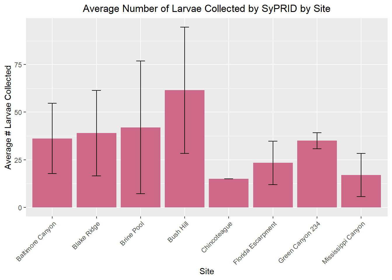

Larval Density

#SDen
SDen$Site <- factor(SDen$Site,levels=c("Baltimore Canyon","Chincoteague","Blake Ridge","Florida Escarpment","Mississippi Canyon","Green Canyon 234","Bush Hill","Brine Pool"))

my_title <- "Average Larval Density Collected by SyPRID by Site"
ggplot(SDen, aes(x=SDen$Site, y=SDen$`Avg Larval Density`,fill=SDen$Site))+geom_bar(stat="identity",position=position_dodge(),width = 0.9)+labs(title =my_title, x="Site", y="Average Larval Density (#/L)")+theme(plot.title = element_text(hjust=0.5), axis.text.x=element_text(angle = 45, vjust = 1, hjust=1))+geom_errorbar(aes(ymin=SDen$`Avg Larval Density`- SDen$`Density STDev...7`, ymax=SDen$`Avg Larval Density`+SDen$`Density STDev...7`), width=.2,position=position_dodge(.9))+scale_fill_viridis_d()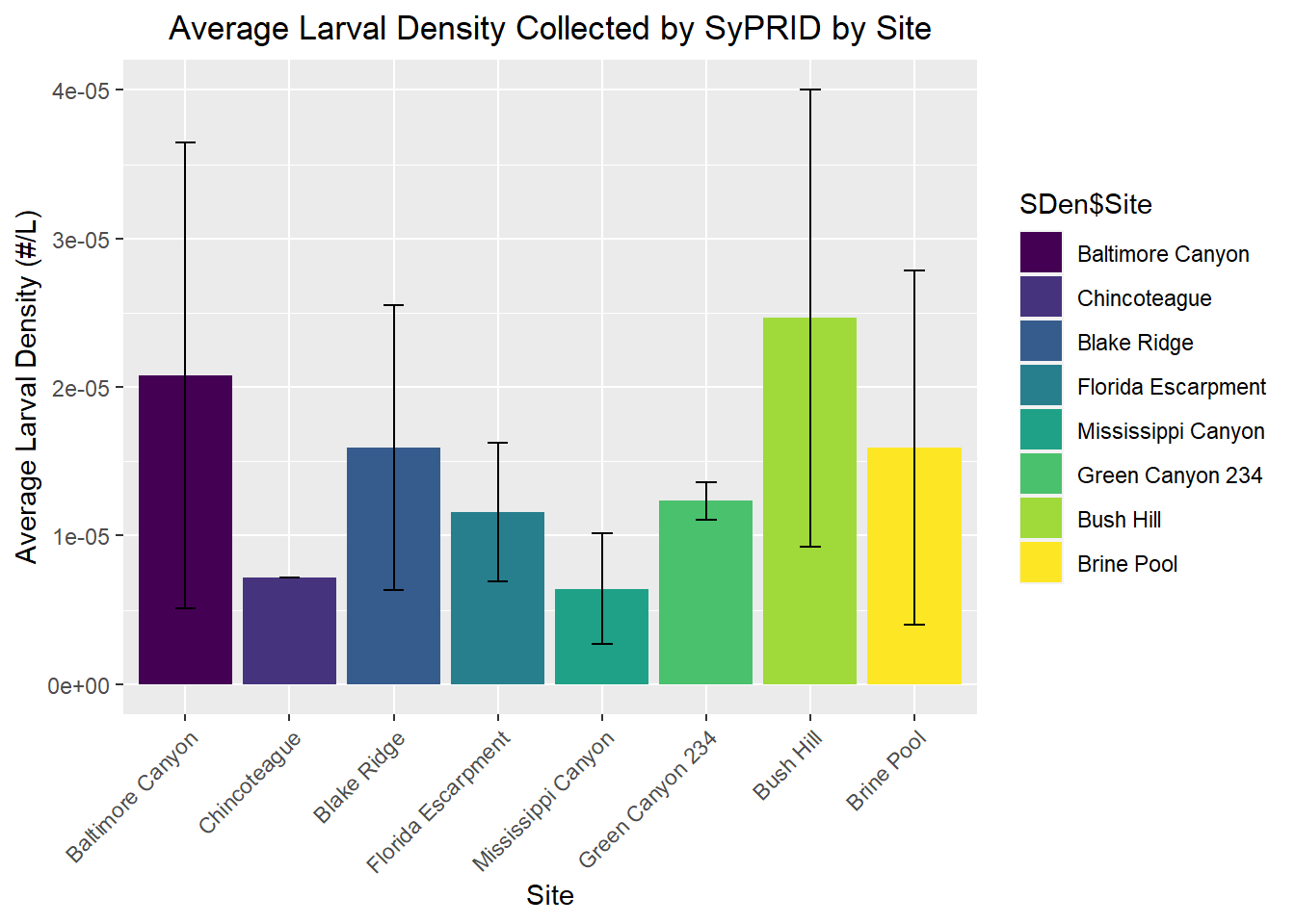

Depth Classifications

Volume Sampled

#DVol
my_title <- "Average Volume of Water Collected by SyPRID by Depth Classification"
ggplot(DVol, aes(x=DVol$`Depth Classification`, y=DVol$`Avg. Volume Sampled (L)`))+geom_bar(fill="deepskyblue3",stat="identity",position=position_dodge(),width = 0.9)+labs(title =my_title, x="Depth", y="Average Volume Collected (L)")+theme(plot.title = element_text(hjust=0.5), axis.text.x=element_text(angle = 45, vjust = 1, hjust=1))+geom_errorbar(aes(ymin=DVol$`Avg. Volume Sampled (L)`- DVol$`Volume STDev...11`, ymax=DVol$`Avg. Volume Sampled (L)`+ DVol$`Volume STDev...11`), width=.2,position=position_dodge(.9))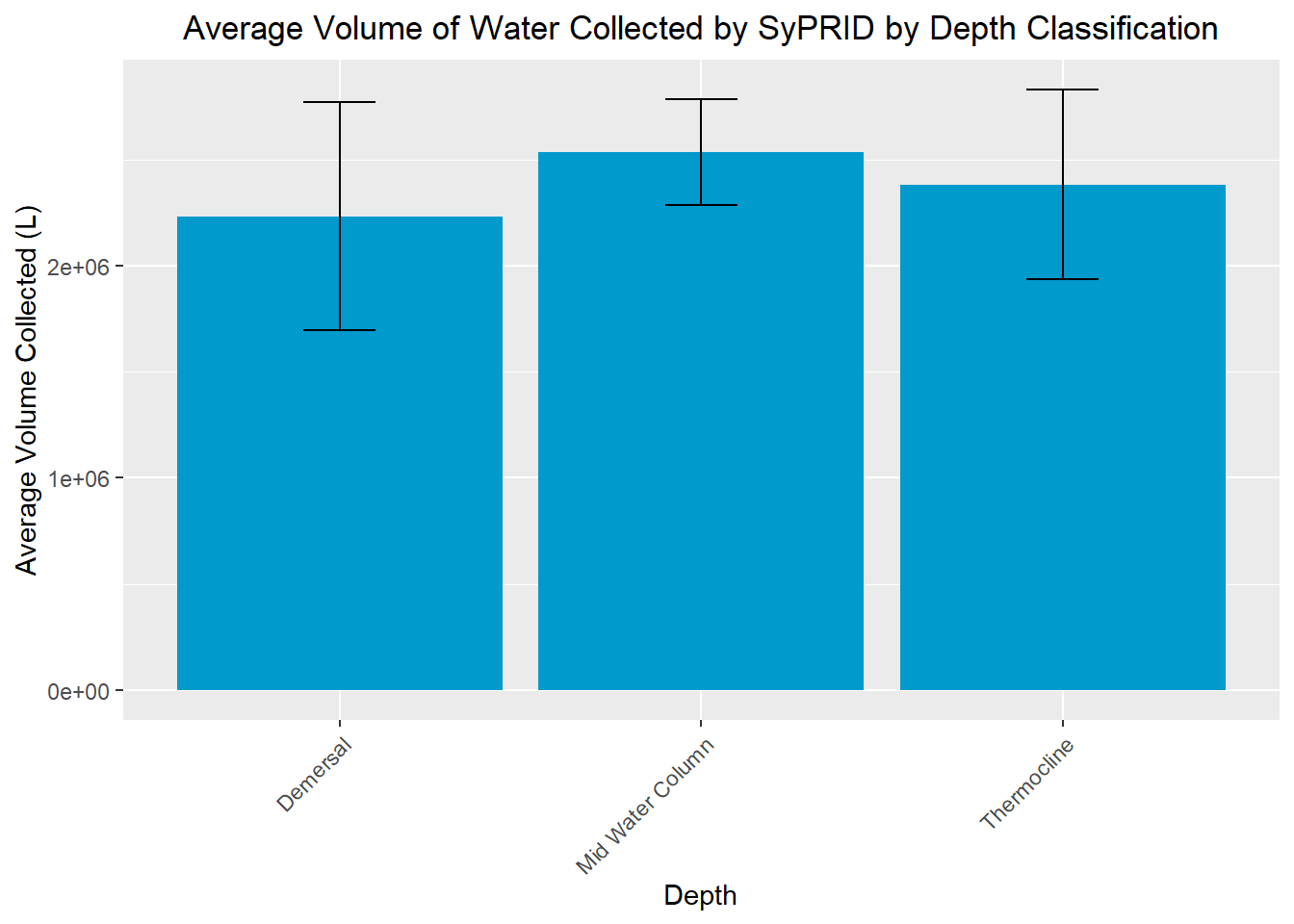

Larvae Collected

#DLar
my_title <- "Average Number of Larvae Collected by SyPRID by Depth Classification"
ggplot(DLar, aes(x=DLar$`Depth Classification`, y=DLar$`Avg. Larvae Collected`))+geom_bar(fill="palevioletred3",stat="identity",position=position_dodge(),width = 0.9)+labs(title =my_title, x="Depth", y="Average # Larvae Collected")+theme(plot.title = element_text(hjust=0.5), axis.text.x=element_text(angle = 45, vjust = 1, hjust=1))+geom_errorbar(aes(ymin=DLar$`Avg. Larvae Collected`- DLar$`Larvae STDev...13`, ymax=DLar$`Avg. Larvae Collected`+DLar$`Larvae STDev...13`), width=.2,position=position_dodge(.9))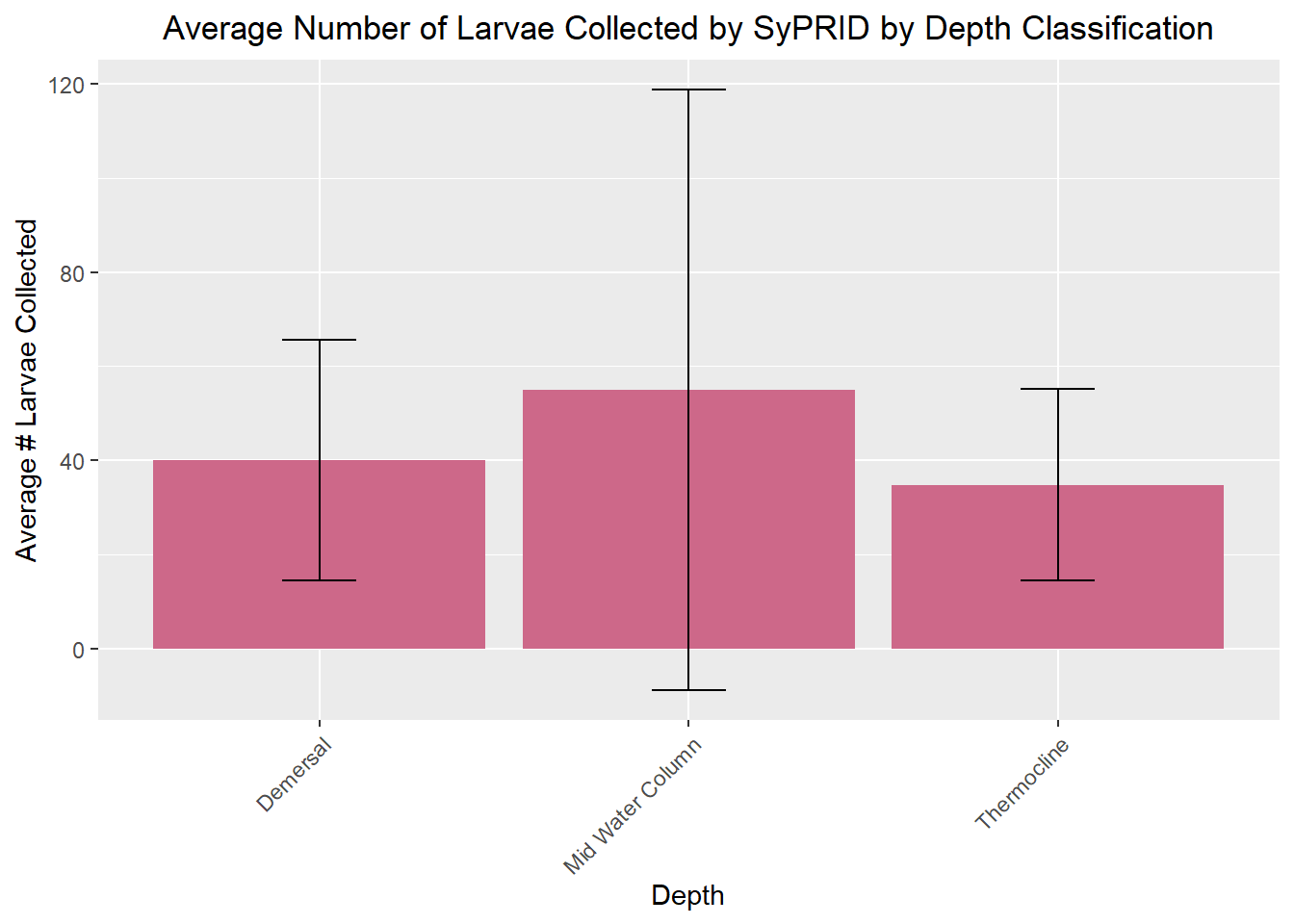

Larval Density

#DDen
my_title <- "Average Larval Density Collected by SyPRID by Depth Classification"
ggplot(DDen, aes(x=DDen$`Depth Classification`, y=DDen$`Avg. Larval Density (#/L)`))+geom_bar(fill=c("darkslategray3","blueviolet","dodgerblue4"),stat="identity",position=position_dodge(),width = 0.9)+labs(title =my_title, x="Site", y="Average Larval Density (#/L)")+theme(plot.title = element_text(hjust=0.5), axis.text.x=element_text(angle = 45, vjust = 1, hjust=1))+geom_errorbar(aes(ymin=DDen$`Avg. Larval Density (#/L)`- DDen$`Density STDev...15`, ymax=DDen$`Avg. Larval Density (#/L)`+DDen$`Density STDev...15`), width=.2,position=position_dodge(.9))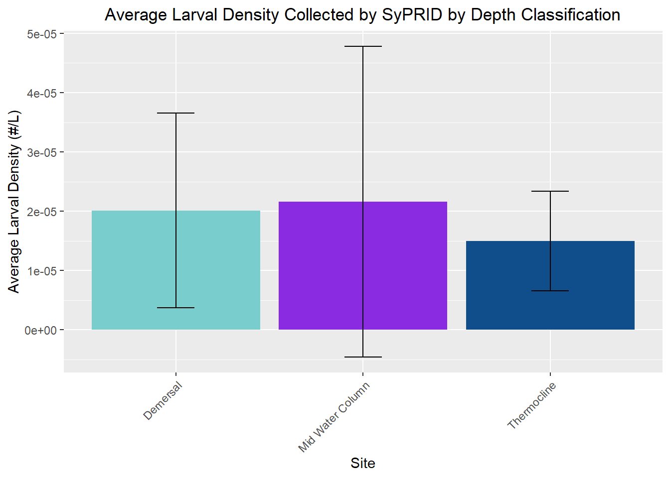

Statistics Within Individual Sites

~~~~~~~~~~~~~~~~~~~~~~~~~~~~~~~~~~~~~~~~~~~~~~

For sites that had multiple dives at given depths (ex. 3 Demersal depths at Brine Pool), the values were averaged resulting in one bar per depth per site.

#Let's make some fuctions!

wrapper <- function(x, ...) 
{
  paste(strwrap(x, ...), collapse = "\n")
}

#Volume Sampled
Vol <- function(site,title){
  ggplot(site, aes(x=`Depth Classification`,y=`Volume Sampled (L)`))+geom_bar(stat="identity", fill='deepskyblue3')+theme(axis.text.x = element_text(angle = 45, vjust = 1, hjust=1))+labs(title=paste0('Volume Sampled with SyPRID by Depth Classificiation at ',title),x="Depth Classificiation", y="Volume Sampled (L)")+theme(plot.title = element_text(hjust = 0.5))
}

#Larvae Collected
Lar <- function(site,title){
  ggplot(site, aes(x=`Depth Classification`,y=`Total Larva Collected`))+geom_bar(stat="identity", fill='palevioletred3')+theme(axis.text.x = element_text(angle = 45, vjust = 1, hjust=1))+labs(title=paste0('Larvae Collected with SyPRID by Depth Classification at ',title),x="Depth Classificiation", y="Number of Larvae")+theme(plot.title = element_text(hjust = 0.5))
}
  
#Larval Density
Den <- function(site,title){
  my_title <- paste0('Larval Density collected with SyPRID by Depth Classification at ',title)
  ggplot(site, aes(x=`Depth Classification`,y=`Larval Density (#/L)`))+geom_bar(stat="identity", fill='salmon2')+theme(axis.text.x = element_text(angle = 45, vjust = 1, hjust=1))+labs(title=my_title ,x="Depth Classificiation", y="Larval Density (#/L)")+theme(plot.title = element_text(hjust = 0.5))+ggtitle(wrapper(my_title, width = 70))
}

Baltimore Canyon

Volume Sampled

Vol(BaltimoreCanyon,"Baltimore Canyon")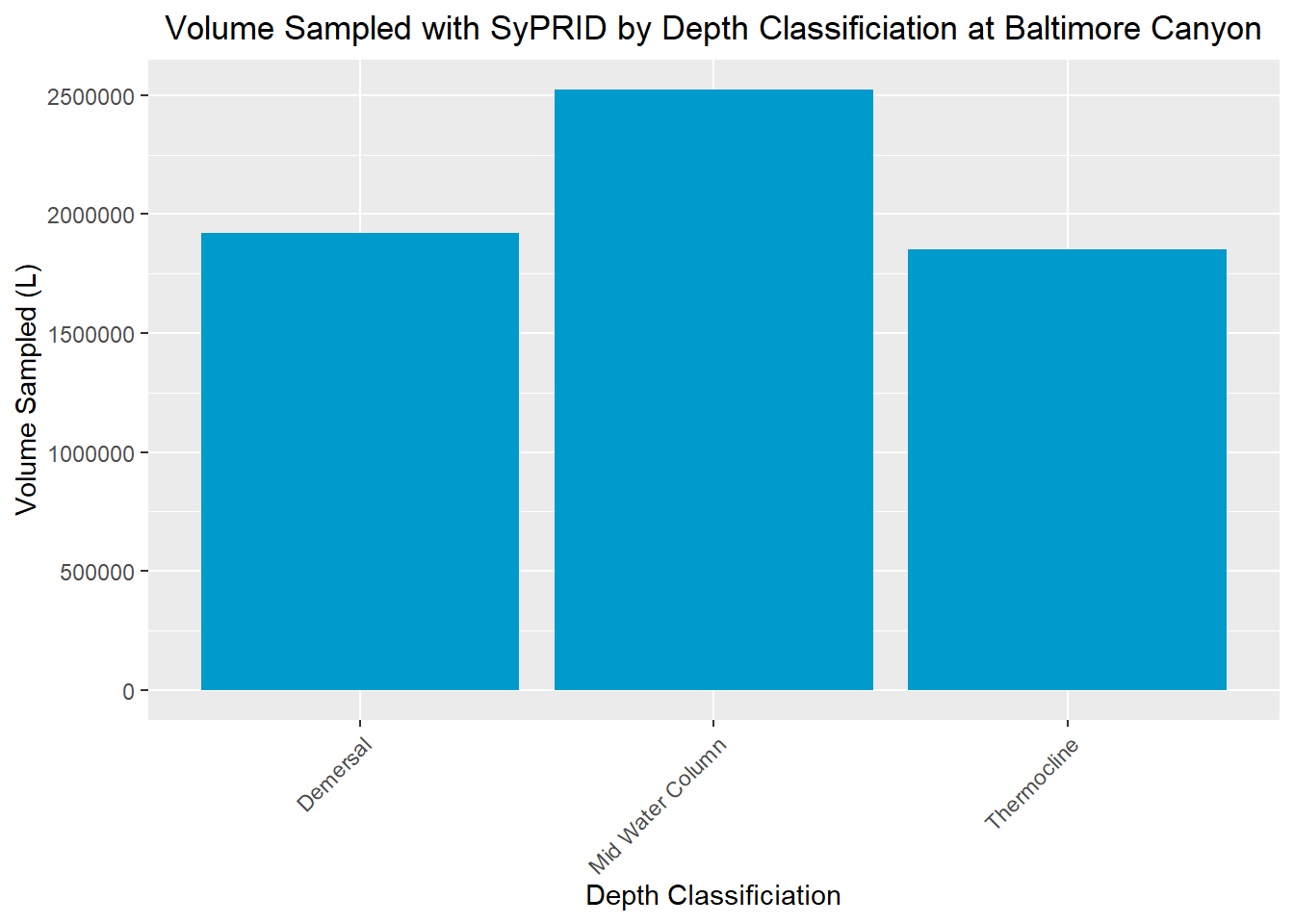

Larvae Collected

Lar(BaltimoreCanyon,"Baltimore Canyon")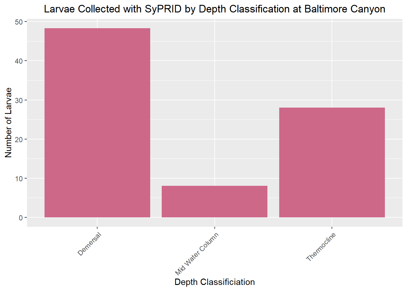

Larval Density

Den(BaltimoreCanyon,"Baltimore Canyon")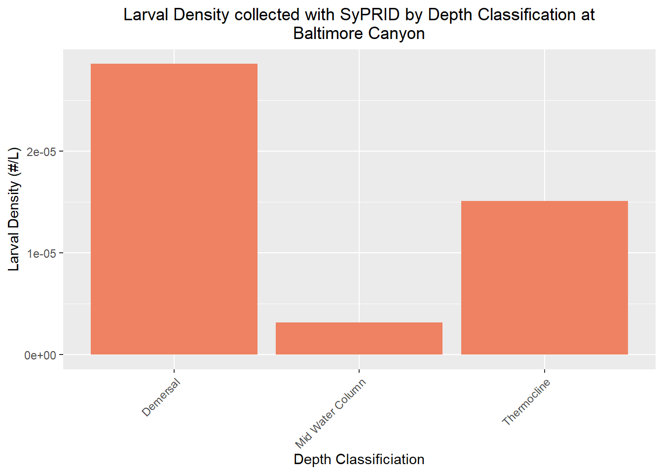

Blake Ridge

Volume Sampled

Vol(BlakeRidge, "Blake Ridge")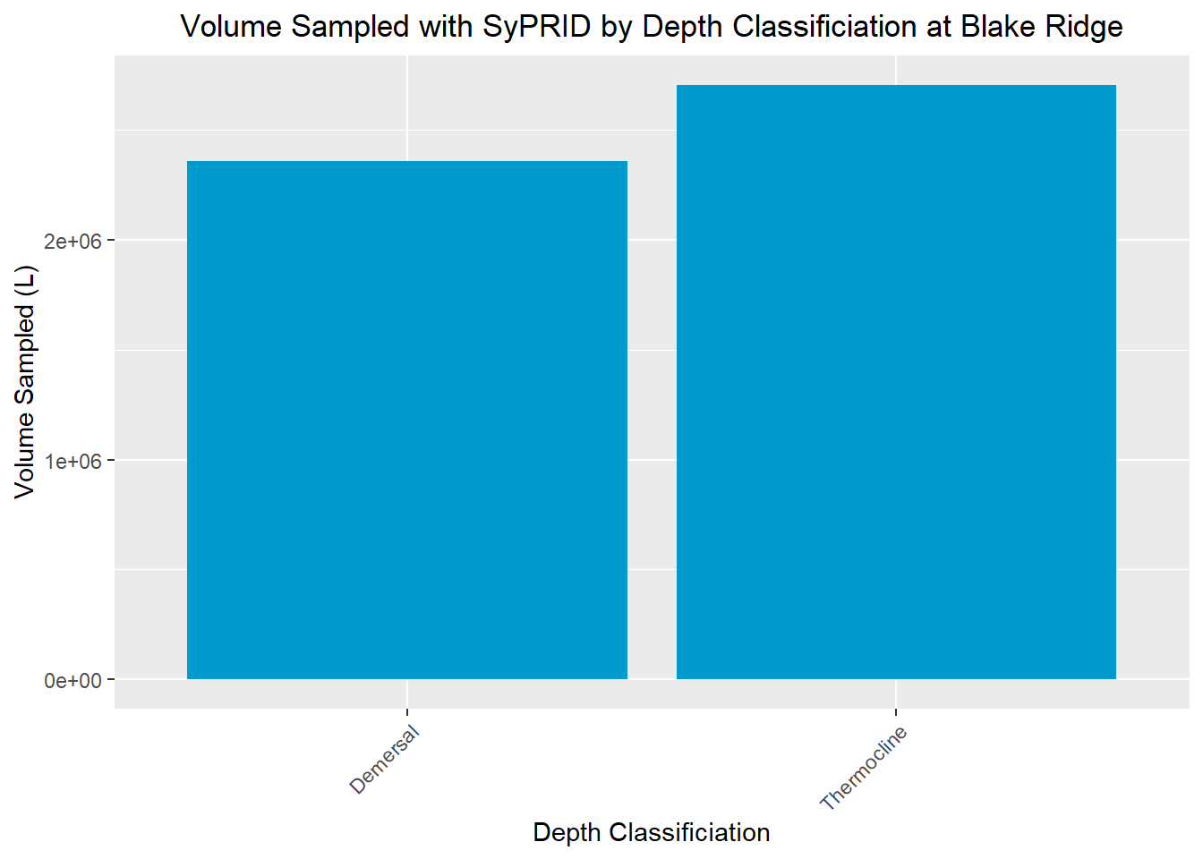

Larvae Collected

Lar(BlakeRidge, "Blake Ridge")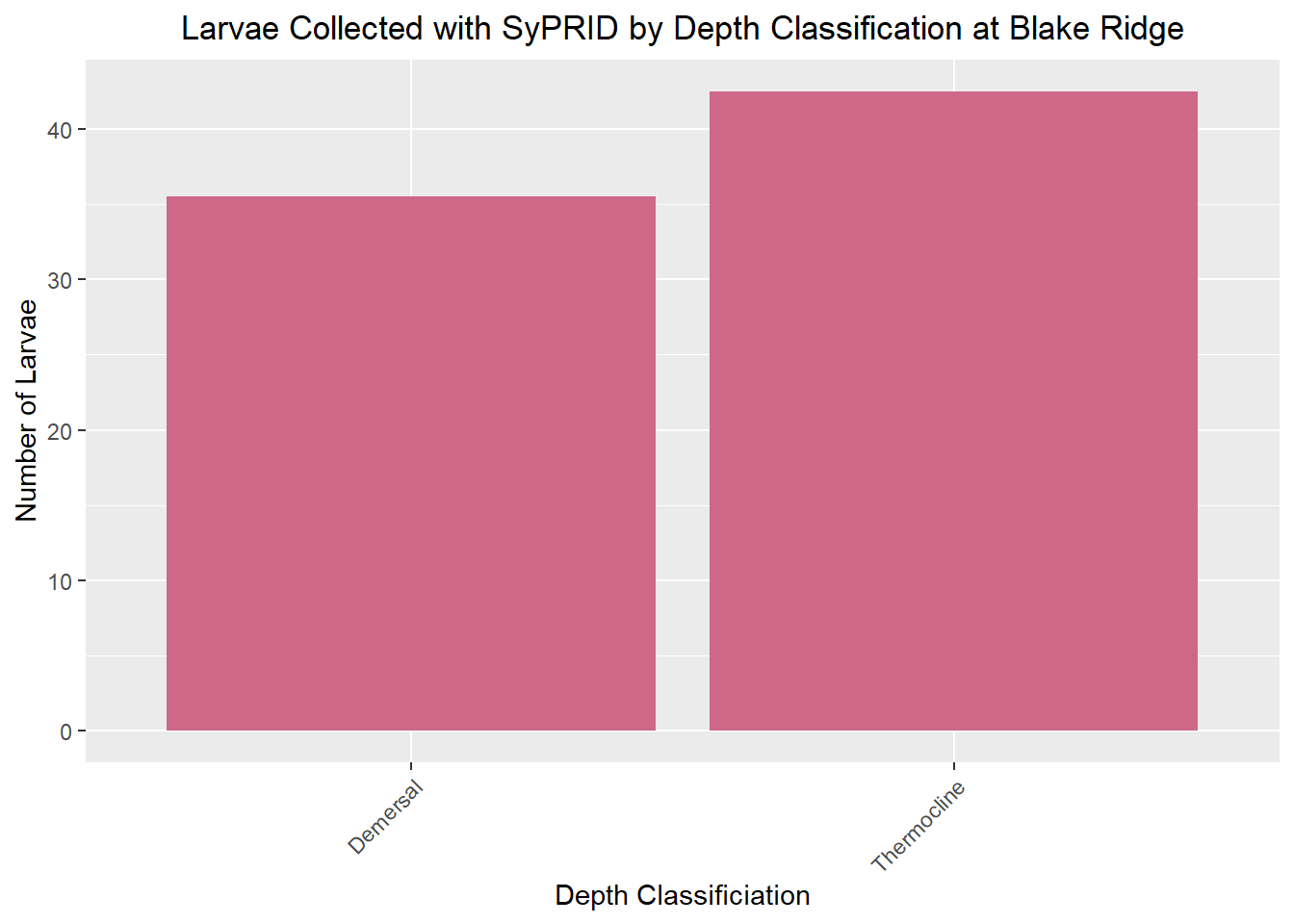

Larval Density

Den(BlakeRidge, "Blake Ridge")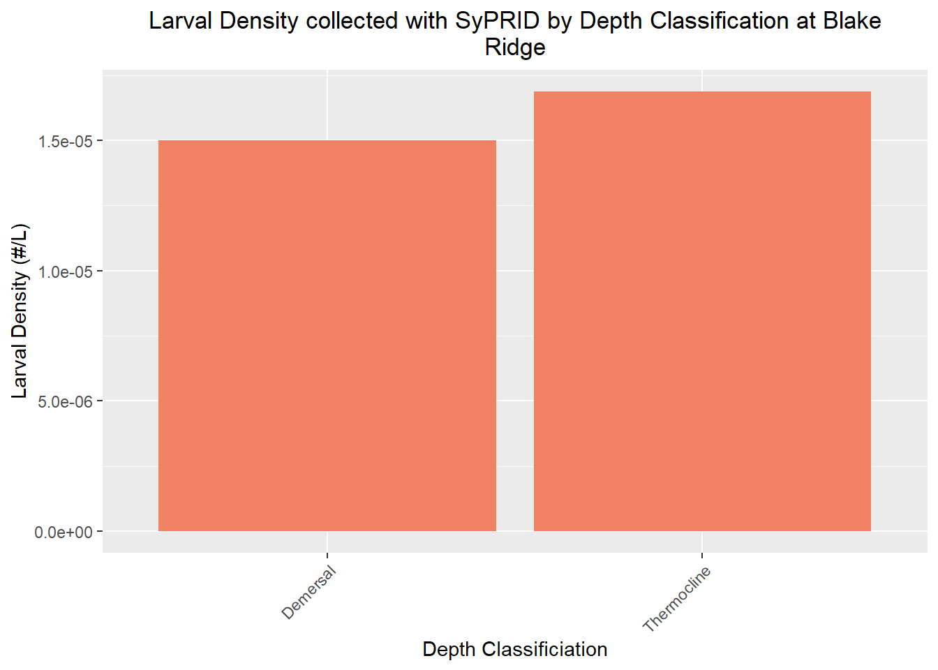

Brine Pool

Volume Sampled

Vol(BrinePool, "Brine Pool")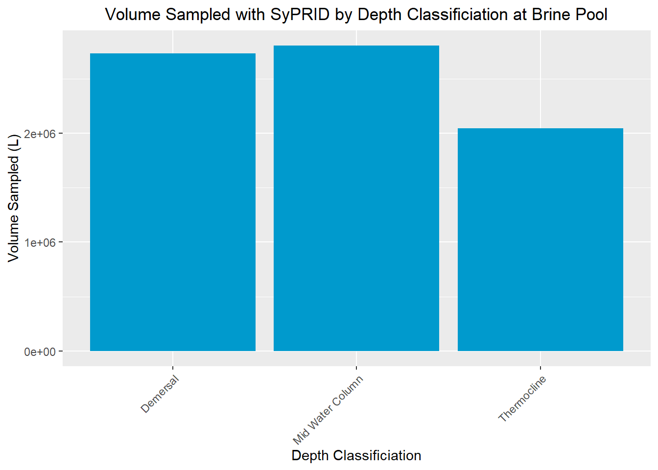

Larvae Collected

Lar(BrinePool, "Brine Pool")

Larval Density

Den(BrinePool, "Brine Pool")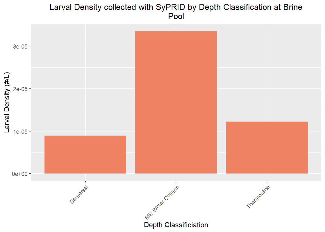

Bush Hill

Volume Sampled

Vol(BushHill, "Bush Hill")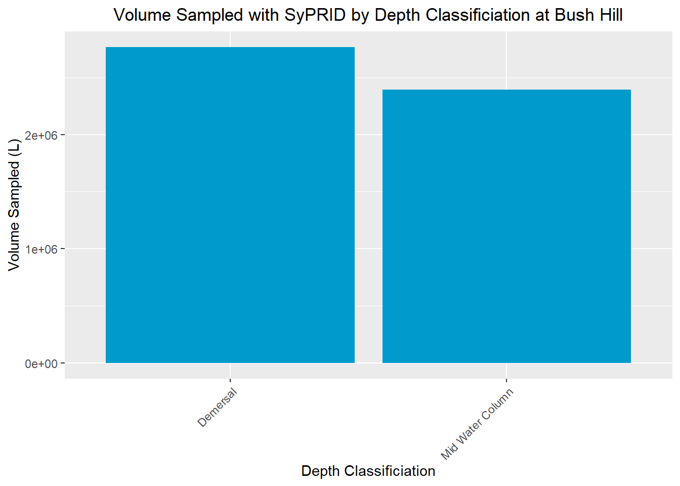

Larvae Collected

Lar(BushHill, "Bush Hill")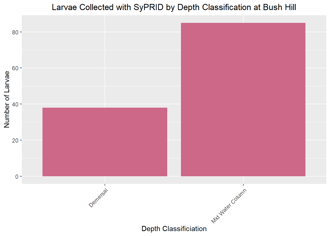

Larval Density

Den(BushHill, "Bush Hill")

Chincoteague

Volume Sampled

Vol(Chincoteague, "Chincoteague")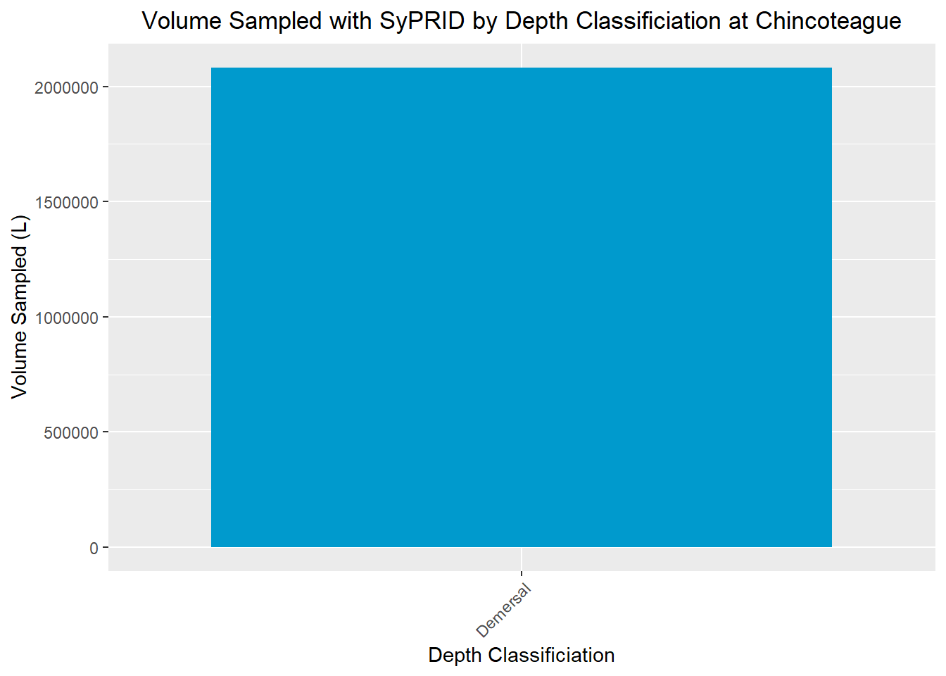

Larvae Collected

Lar(Chincoteague, "Chincoteague")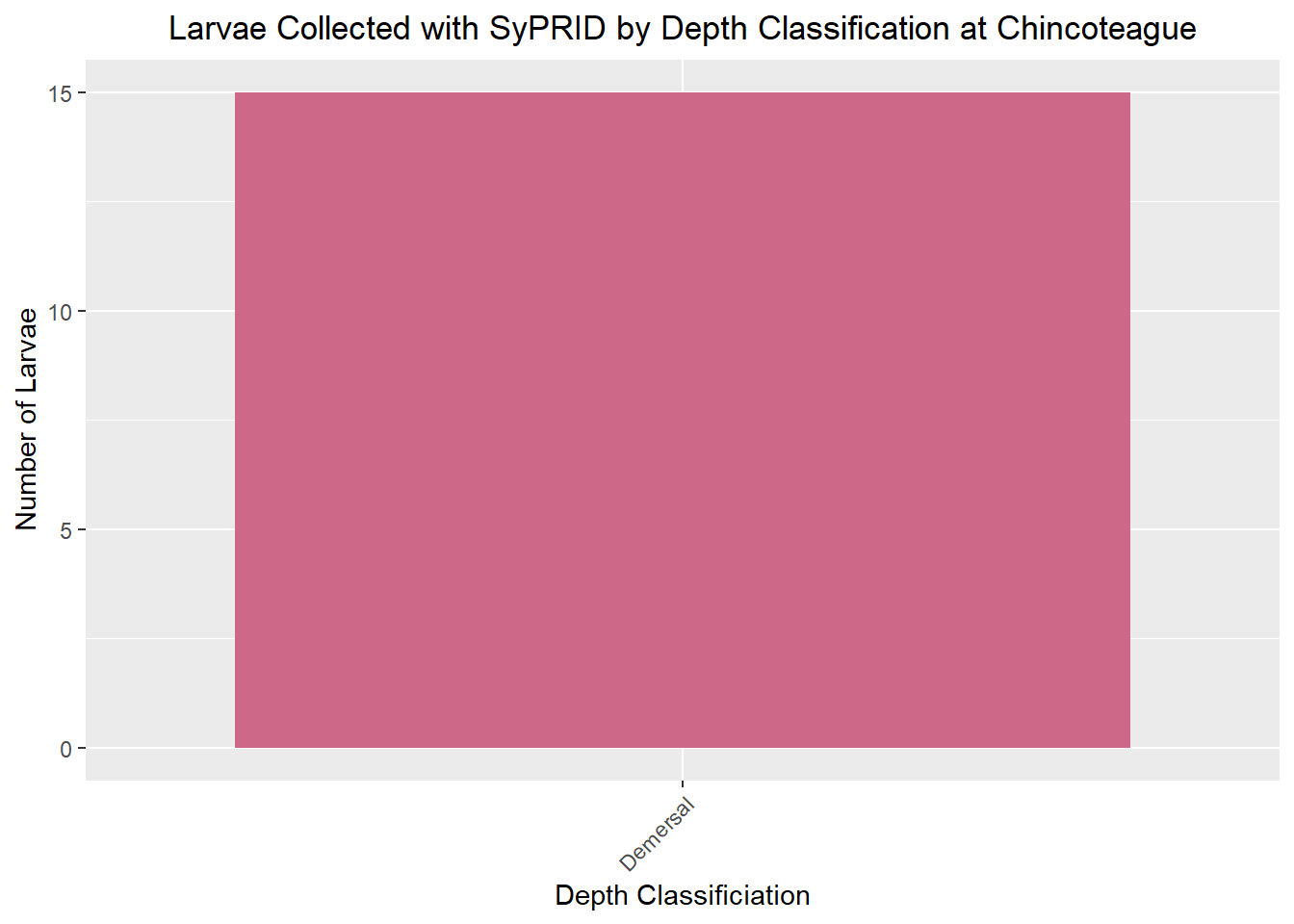

Larval Density

Den(Chincoteague, "Chincoteague")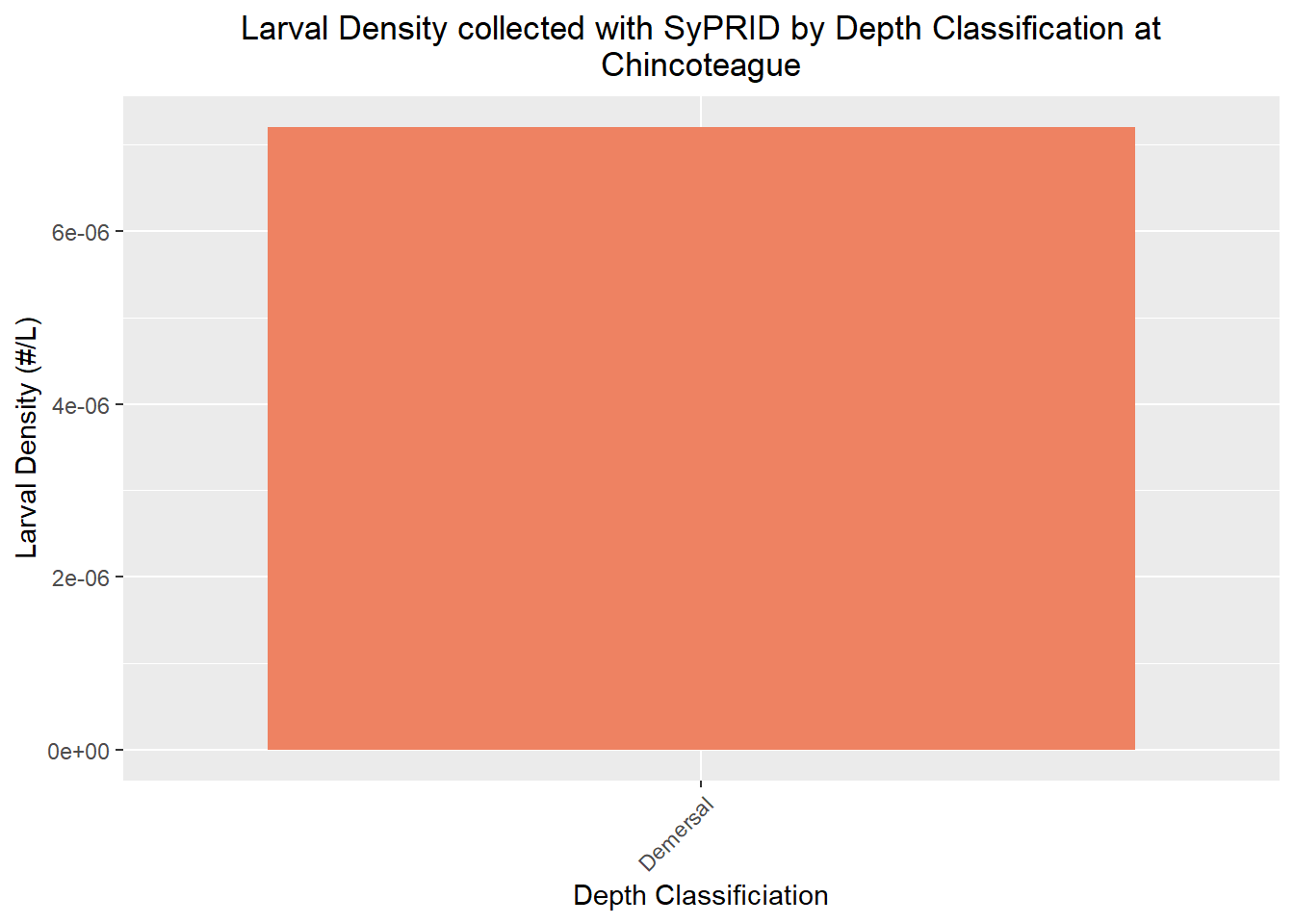

Florida Escarpment

Volume Sampled

Vol(FloridaEscarpment, "Florida Escarpment")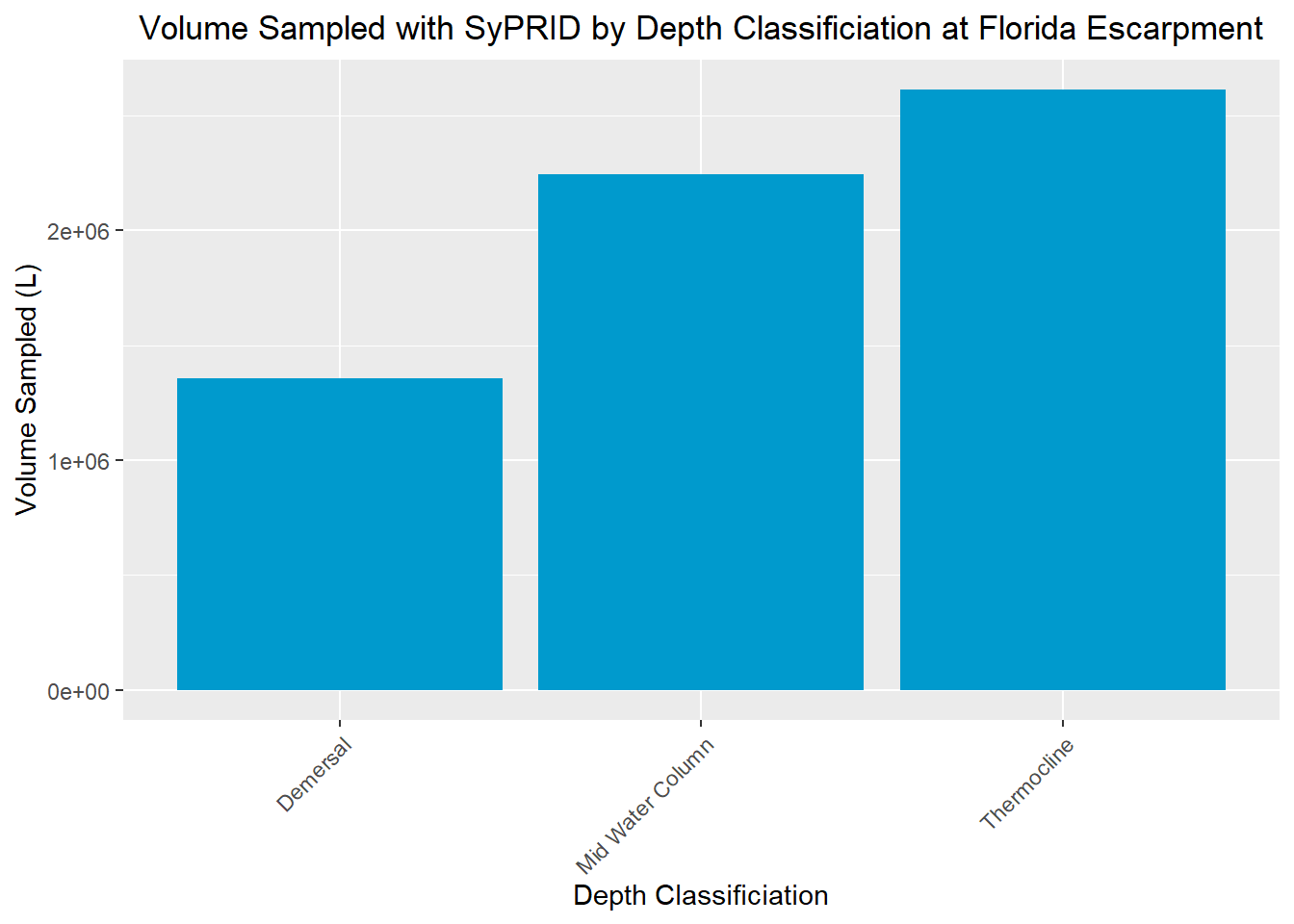

Larvae Collected

Lar(FloridaEscarpment, "Florida Escarpment")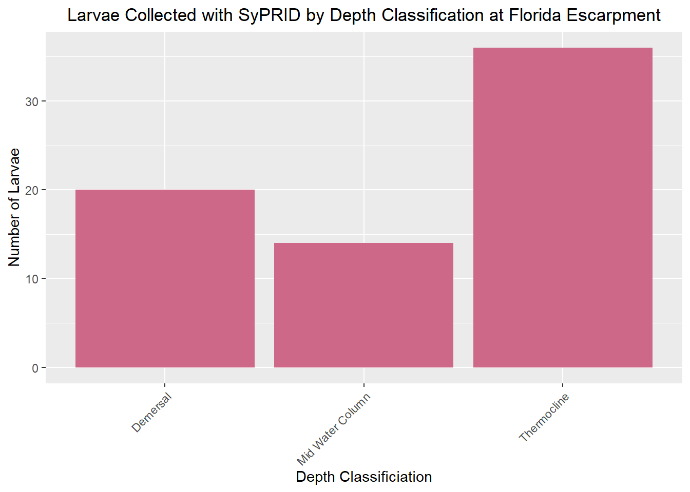

Larval Density

Den(FloridaEscarpment, "Florida Escarpment")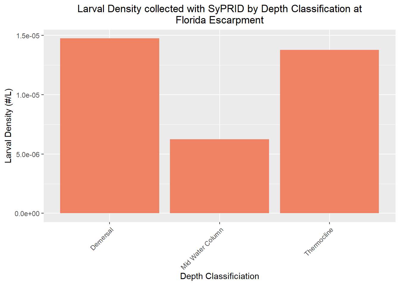

Green Canyon 234

Volume Sampled

Vol(GC234, "Green Canyon 234")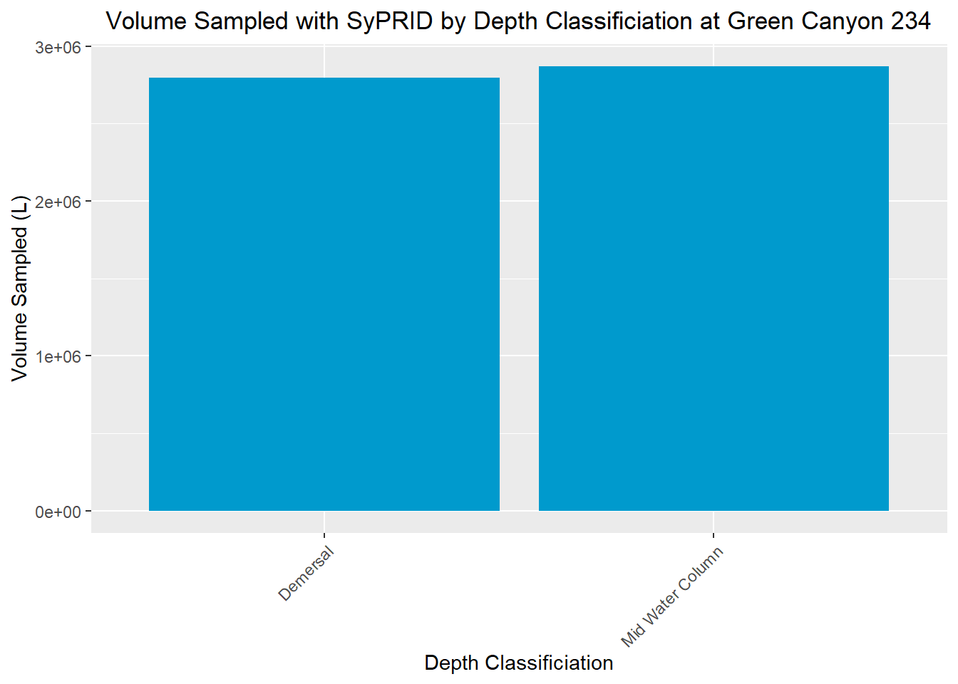

Larvae Collected

Lar(GC234, "Green Canyon 234")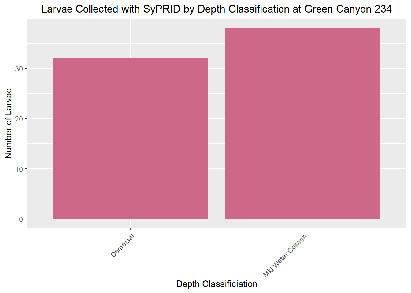

Larval Density

Den(GC234, "Green Canyon 234")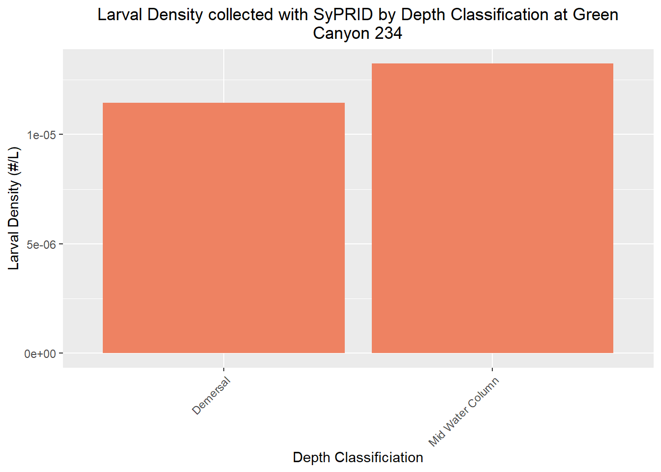

Mississippi Canyon

Volume Sampled

Vol(MississippiCanyon, "Mississippi Canyon")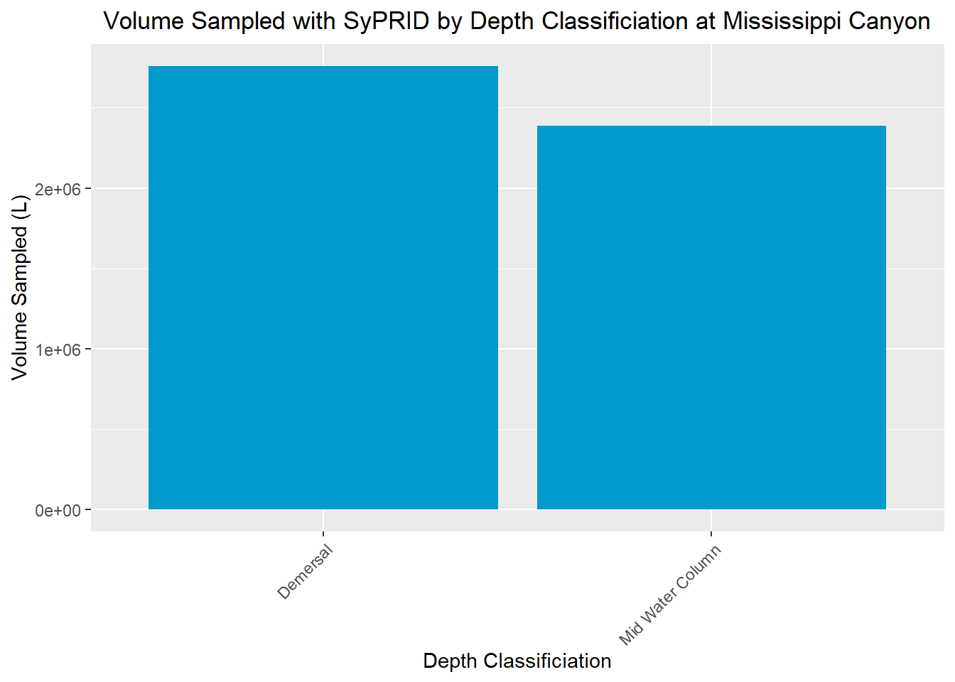

Larvae Collected

Lar(MississippiCanyon, "Mississippi Canyon")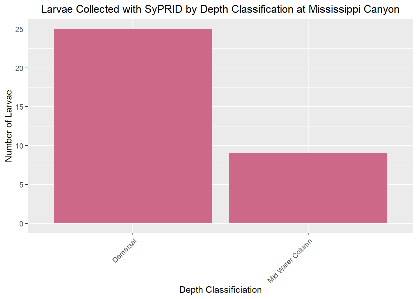

Larval Density

Den(MississippiCanyon, "Mississippi Canyon")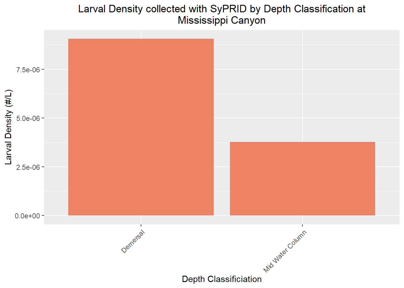

Morphotyping Results

Larval Type Guide

~~~~~~~~~~~~~~~~~~~~~~~~~~~~~~~~~~~~~~~~~~~~~~

SALT Larval Types Found
Form	Phylum	Morphotype Name
AC	Phoronida	Actinotroph
AJ	Echinodermata	Asteroid Juvenile
AT	Cnidaria	Actinula
AU	Echinodermata	Auricularia
BL	Echinodermata	Brachiolaria
BP	Echinodermata	Bipinnaria
BV	Mollusca	Bivalve Veliger
CB	Ctenophora	Cydippid
CE	Cnidaria	Cerinula
CP	Arthropoda	Cyprid
CY	Bryozoa	Cyphonautes
DL	Echinodermata	Doliolaria
EC	Annelida	Echiura
EP	Cnidaria	Ephyra
GV	Mollusca	Gastropod Veliger
LG	Brachiopoda	Lingula
MI	Annelida	Mitraria
ML	Arthropoda	Megalopa
NE	Annelida	Nectochaete
NP	Arthropoda	Nauplius
OJ	Echinodermata	Ophiuroid Juvenile
OP	Echinodermata	Ophiopluteus
PC	Porifera	Parenchymula
PG/PS	Annelida	Pelagosphera
PI	Nemertea	Pilidium
PL	Cnidaria	Planula
PU	Echinodermata	Pluteus
SQ	Mollusca	Squid Paralarva
ST	Annelida	Setiger
TO	Hemichordata	Tornaria
TP	Annelida / Mollusca	Trocophore
UJ	Echinodermata	Urchin Juvenile
ZE	Cnidaria	Zoanthella
ZO	Arthropoda	Zoea

Larval Type Presence by Depth

~~~~~~~~~~~~~~~~~~~~~~~~~~~~~~~~~~~~~~~~~~~~~~

Demersal

Larval Types Found at Demersal Depths
Site	Dive	# Morphotypes	Larval Types Present
Baltimore Canyon	S583P	8	BV/GV/NP/PC/PG/TP/ZO
Baltimore Canyon	S584P	8	BV/GV/PC/PG/PL/TP/ZO
Baltimore Canyon	S585P	8	BV/CY/PC/PL/TP/ZO
Blake Ridge	S587P	7	BV/CY/GV/MI/NE/TP
Blake Ridge	S588P	7	BV/GV/NE/OP
Brine Pool	S572S	12	BP/BV/GV/NE/NP/OJ/TP
Brine Pool	S592P	13	BV/GV/NE/OJ/PL
Brine Pool	S593P	11	AT/BL/BV/CY/GV/NE
Bush Hill	S594P	11	AT/BL/BV/GV/LG/NE/OJ/TP
Chincoteague	S592P	5	DL/NE/NP/TP/ZO
Florida Escarpment	S589P	9	BV/CY/NE/NP
Green Canyon 234	S591P	12	BV/CY/GV/ML/NE/ZO
Mississippi Canyon	S595P	7	BV/DL/GV/LG/TP

Mid Water Column

Larval Types Found at Mid Water Column Depths
Site	Dive	# Morphotypes	Larval Types Present
Baltimore Canyon	S584S	5	CY/GV/NE/PL/TP
Brine Pool	S592S	13	AT/BV/CY/GV/NE/OK/PC/PL/TP
Bush Hill	S594S	11	AT/BV/CY/GV/MI/NE/OJ/OP/PL
Florida Escarpment	S590S	5	BV/CY/GV/NE
Green Canyon 234	S591S	11	BL/BV/CY/GV/LG/NE/TP
Mississippi Canyon	S595S	4	AT/GV/NE/TP

Thermocline

Larval Types Found at Thermocline Depths
Site	Dive	# Morphotypes	Larval Types Present
Baltimore Canyon	S583S	9	BV/GV/ML/PC/PG/PL/TP/ZO
Blake Ridge	S587S	7	AT/BV/CY/GV/PG/TP
Blake Ridge	S588S	8	BV/CY/MI/PG/PI/PL
Brine Pool	S593S	9	BL/BV/CY/DL/GV/NE/OJ
Florida Escarpment	S589S	9	BV/GV/MI/NE/PG/TP

Larval Types Present in Every Depth Classification*:

Community Composition Analysis

~~~~~~~~~~~~~~~~~~~~~~~~~~~~~~~~~~~~~~~~~~~~~~

NMDS Plot

SALT <- read_xlsx("SALT_Larval_Consensus_Final-COPY.xlsx", sheet = "Morphotype Counts by Depth")
SALT <- subset(SALT, SALT$Method == "Sentry") #Only interested in Sentry Data
SALT <- subset(SALT, SALT$Site != "Florida Keys") #Not using Florida Keys Samples
SALT <- subset(SALT, SALT$Cruise != "EN658")

#NMDS Data Analysis

NMDS <- metaMDS(SALT[c(11:151,153:154)], k=2) #Removed unkown (UNK) Morphotype

## Square root transformation
## Wisconsin double standardization
## Run 0 stress 0.2082584 
## Run 1 stress 0.2249806 
## Run 2 stress 0.2082584 
## ... New best solution
## ... Procrustes: rmse 7.123955e-06  max resid 1.933612e-05 
## ... Similar to previous best
## Run 3 stress 0.2577065 
## Run 4 stress 0.2082584 
## ... New best solution
## ... Procrustes: rmse 9.227413e-06  max resid 2.285938e-05 
## ... Similar to previous best
## Run 5 stress 0.2249805 
## Run 6 stress 0.2082983 
## ... Procrustes: rmse 0.01469259  max resid 0.04988133 
## Run 7 stress 0.2125757 
## Run 8 stress 0.2113348 
## Run 9 stress 0.2082584 
## ... Procrustes: rmse 6.004551e-06  max resid 1.471178e-05 
## ... Similar to previous best
## Run 10 stress 0.2370726 
## Run 11 stress 0.2478411 
## Run 12 stress 0.2113348 
## Run 13 stress 0.2466424 
## Run 14 stress 0.2082983 
## ... Procrustes: rmse 0.01465319  max resid 0.04974242 
## Run 15 stress 0.2082983 
## ... Procrustes: rmse 0.01466932  max resid 0.04980125 
## Run 16 stress 0.2367192 
## Run 17 stress 0.2082584 
## ... Procrustes: rmse 9.743249e-06  max resid 2.097695e-05 
## ... Similar to previous best
## Run 18 stress 0.2113348 
## Run 19 stress 0.2459374 
## Run 20 stress 0.2100642 
## *** Solution reached

#Creating a data frame with the NMDS values
data.scores <- as.data.frame(scores(NMDS,NMDS$sites)) #Using scores functions from Vegan to extract NMDS values into data frame
data.scores$Site <- SALT$Site #Site Information from SALT Spreadsheet
data.scores$Cruise <- SALT$Cruise # Cruise EN658 or TN391
data.scores$Depth <- SALT $`Depth Classification` # Depth Classification - Demersal, Low WC, Mid WC, Thermocline

depth <- data.scores$Depth
site <- data.scores$Site
stress <-mean(round(NMDS$stress,digits=1)) 
p2 <- ggplot() + 
  geom_point(data=data.scores,aes(x=NMDS1,y=NMDS2,shape=data.scores$Depth, color=data.scores$Site), size=4) + # add the point markers
  coord_equal() +  scale_color_manual(values=c("Baltimore Canyon" = "firebrick1", "Blake Ridge" = "forest green", "Brine Pool" = "blue", "Bush Hill" = "orange", "Chincoteague" = "darkgoldenrod4", "Florida Escarpment" = "plum2", "Green Canyon 234" = "purple3", "Mississippi Canyon" = "cyan4"), name = "Site") +
  scale_shape_manual(values=c("Demersal" = 15, "Mid Water Column" = 17, "Thermocline" = 19), name = "Depth Classification") +
  guides(fill = guide_legend(order = 1, override.aes = list(shape = NA, alpha = 1)), shape = guide_legend(order = 2)) +
  theme_classic() + 
  theme(panel.border = element_rect(colour = "black", fill = NA), 
        axis.text.x = element_text(size=12, colour="black"),  axis.text.y = element_text(size=12, colour="black"), 
        axis.title.x = element_text(size=14, colour="black"), axis.title.y = element_text(size=14, colour="black"))+annotate("text",x=-0.5,y=.7,label=paste("Stress =",stress))
p2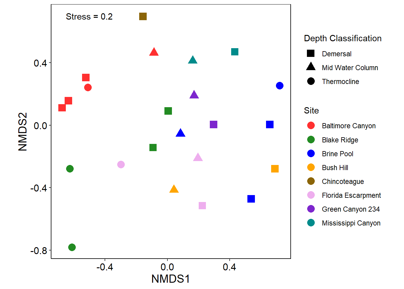

Dendogram

test.dist<-vegdist(SALT[c(11:151,153:154)], method="bray")
cluster.circles<-hclust(test.dist, method="average") 
plot(cluster.circles, ylab="Dissimilarity OR 1-Similarity",labels=SALT$`Depth Classification`,hang=-.1, xlab="")
abline(h=.30,lty=3)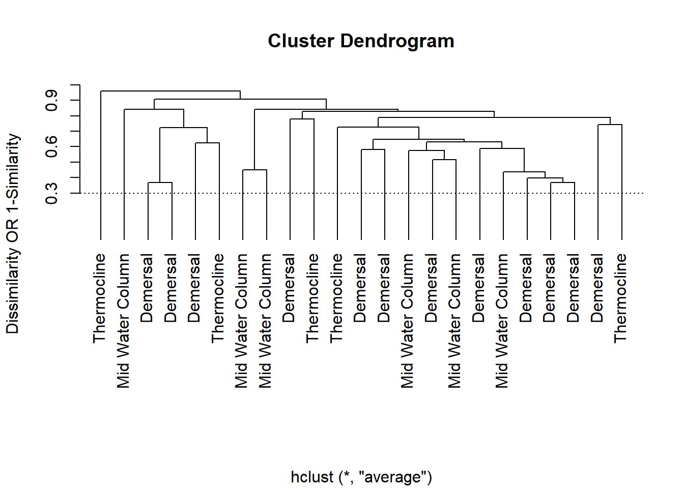

##{-}

Morphotype Proportion by Depth and Site

~~~~~~~~~~~~~~~~~~~~~~~~~~~~~~~~~~~~~~~~~~~~~~

Significant Morphotypes

# Heat Map of Bivalve Veliger Morphotypes.
HeatDat <- read_xlsx("Morphotype_Consensus_Percentages.xlsx", sheet = "Final")
HeatDat <- subset(HeatDat, HeatDat$Cruise == "TN391")
HeatMat <- HeatDat[-c(1:6,35)]
mypalette <- colorRampPalette(c("white","slateblue1","slateblue4"))(n=1000)


Sig <- HeatMat[-c(1:2,6:8,11:17,19:21,23,26:28)]
rownames(Sig) <- c(HeatDat$`Sample Name`)


heat <- as.matrix(Sig)
heat <-t(heat)
heatmap.2(heat,
          symkey = FALSE, 
          Rowv = FALSE,
          Colv = FALSE,
          xlab = "Site", 
          ylab="Morphotype", 
          ColSideColors = c('dodgerblue4','darkslategray3','cyan2','dodgerblue4','dodgerblue4','cyan2','dodgerblue4','darkslategray3','cyan2','dodgerblue4','darkslategray3','dodgerblue4','darkslategray3','cyan2','dodgerblue4','darkslategray3','dodgerblue4','darkslategray3'),
          col = mypalette,
          add.expr = c(abline(v=6.5),
          col = c("cyan","darkslategray3","dodgerblue4"),pch=19), 
          trace="none", 
          density.info = "none", 
          key.xlab = "Proportion of Larval Sample")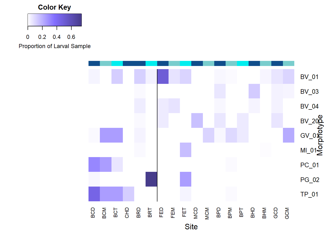

All Morphotypes

# Heat Map of Bivalve Veliger Morphotypes.
HeatDat <- read_xlsx("Morphotype_Consensus_Percentages.xlsx", sheet = "Final")
HeatDat <- subset(HeatDat, HeatDat$Cruise == "TN391")
HeatMat <- HeatDat[-c(1:6,35)]
mypalette <- colorRampPalette(c("white","slateblue1","slateblue4"))(n=1000)

row.names(HeatMat) <-  (HeatDat$`Sample Name`)
heat <- as.matrix(HeatMat)
heat <-t(heat)
heatmap.2(heat,
          symkey = FALSE, 
          Rowv = FALSE,
          Colv = FALSE,
          xlab = "Site", 
          
          ylab="Morphotype", 
          ColSideColors = c('dodgerblue4','darkslategray3','cyan2','dodgerblue4','dodgerblue4','cyan2','dodgerblue4','darkslategray3','cyan2','dodgerblue4','darkslategray3','dodgerblue4','darkslategray3','cyan2','dodgerblue4','darkslategray3','dodgerblue4','darkslategray3'),
          col = mypalette, 
          add.expr = c(abline(v=6.5),
          col = c("cyan","darkslategray3","dodgerblue4"),pch=19), 
          trace="none", 
          density.info = "none", 
          key.xlab = "Proportion of Larval Sample")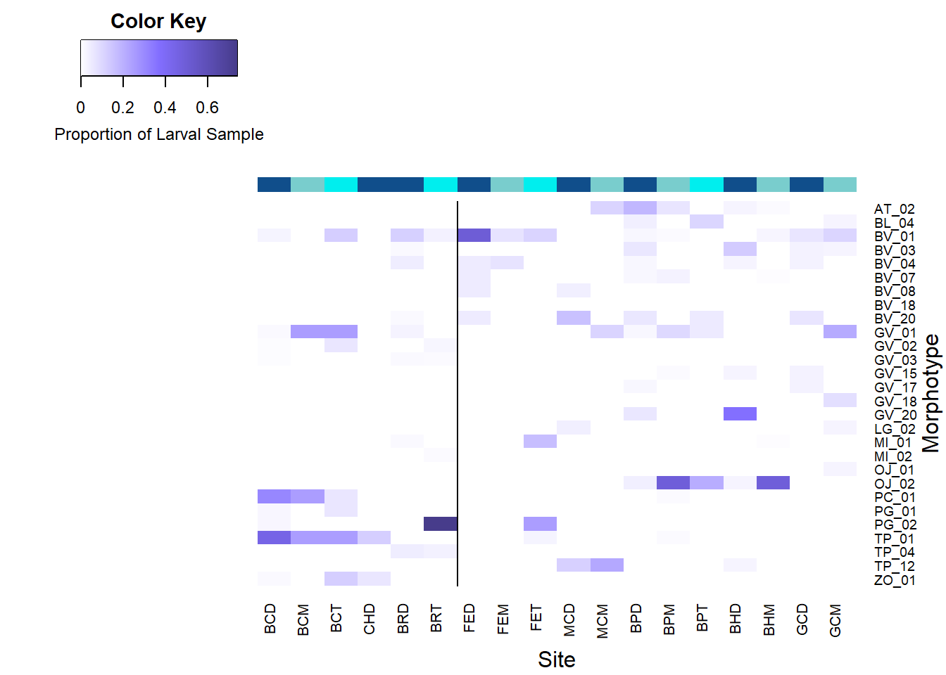

Brine Pool Seasonality

# Heat Map of Bivalve Veliger Morphotypes.
HeatDat <- read_xlsx("Morphotype_Consensus_Percentages.xlsx", sheet = "Final")
HeatDat <- subset(HeatDat, HeatDat$Site == "Brine Pool")
HeatMat <- HeatDat[-c(1:6,13,17:18,24,29,32:34,35)]
mypalette <- colorRampPalette(c("white","slateblue1","slateblue4"))(n=1000)

row.names(HeatMat) <-  (c("FallD","FallM","SpringD","SpringM","SpringT"))
heat <- as.matrix(HeatMat)
heat <-t(heat)
heatmap.2(heat,
          symkey = FALSE, 
          Rowv = FALSE,
          Colv = FALSE,
          xlab = "Site", 
          
          ylab="Morphotype", 
          ColSideColors = c('dodgerblue4','darkslategray3','dodgerblue4','darkslategray3','cyan2'),
          col = mypalette, 
          add.expr = c(abline(v=2.5),
          col = c("cyan","darkslategray3","dodgerblue4"),pch=19), 
          trace="none", 
          density.info = "none", 
          key.xlab = "Proportion of Larval Sample",
          srtCol=45)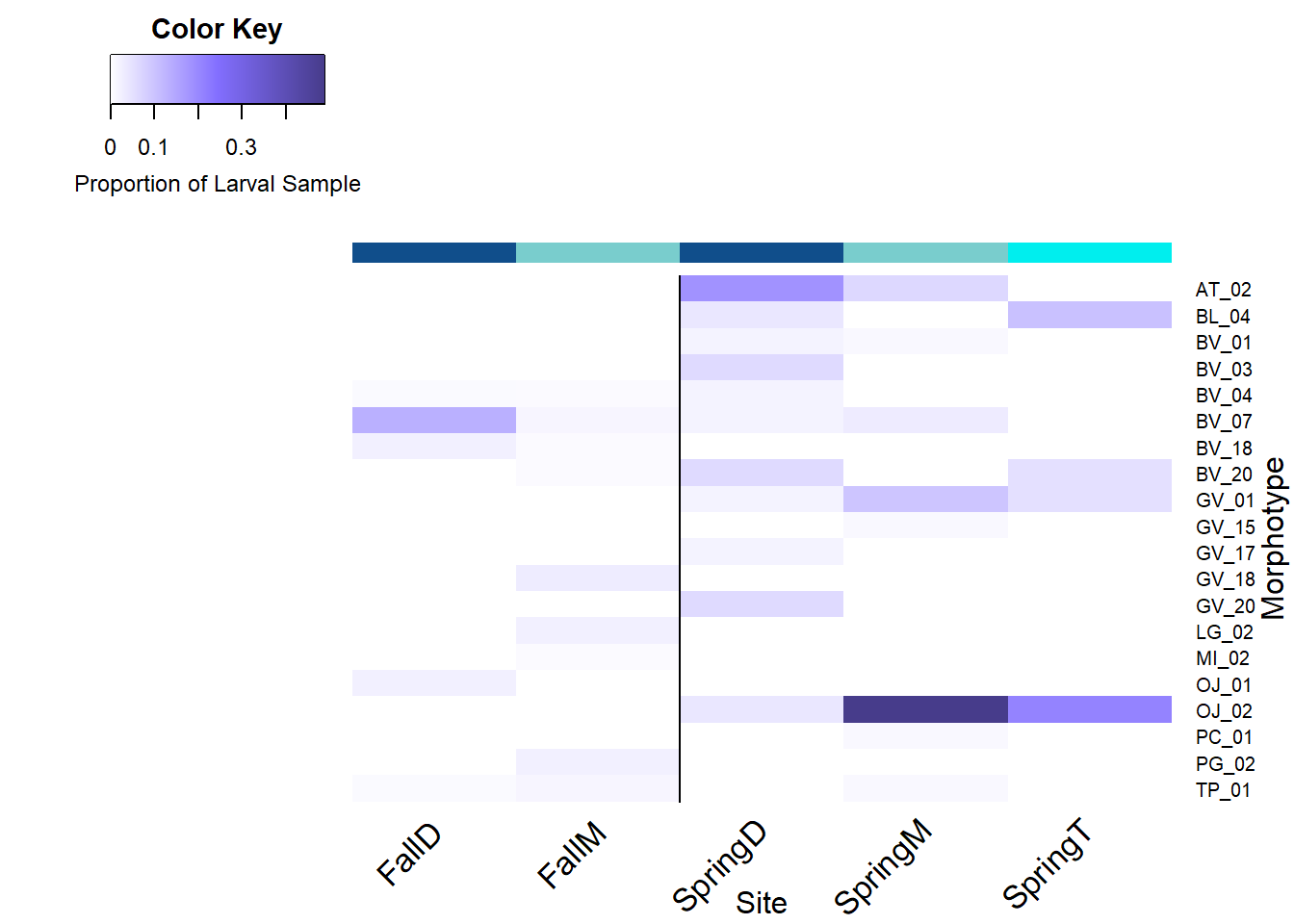

* Site codes denote the following: BC = Baltimore Canyon, CH = Chincoteague, BR = Blake Ridge, FE = Florida Escarpment, MC = Mississippi Canyon, BP = Brine Pool, BH = Bush Hill, GC = Green Canyon 234. The letters after these site codes represent the depth classificaiton; D = Demersal, M = Mid Water Column, T = Thermocline.

For Brine Pool, collections from the Fall 2020 EN658 cruise are denoted with the codes Fall, while the other site codes are from the Spring 2021 TN391 cruise.

The color bar along the columns acts as a visual aid for the depth classifications; demersal ( darkblue ), mid water column ( gray-blue ), thermocline ( cyan ).

The vertical line represents the geographical split between the Western Atlantic Margin (left) and the Gulf of Mexico (right) sites or the split between Fall and Spring cruises.

Total Counts for Depth Classifications (Notes)

~~~~~~~~~~~~~~~~~~~~~~~~~~~~~~~~~~~~~~~~~~~~~~

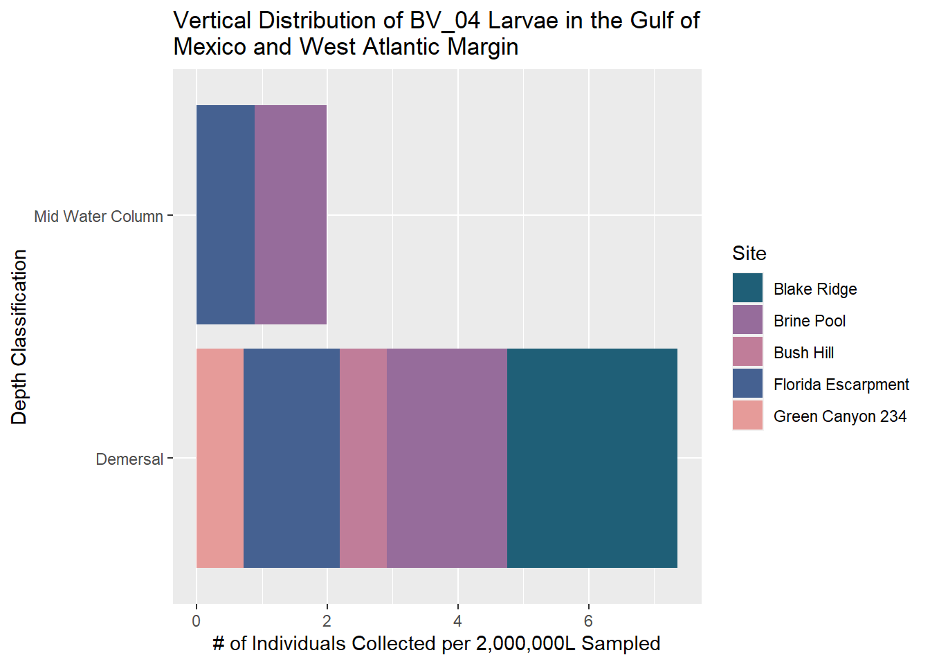
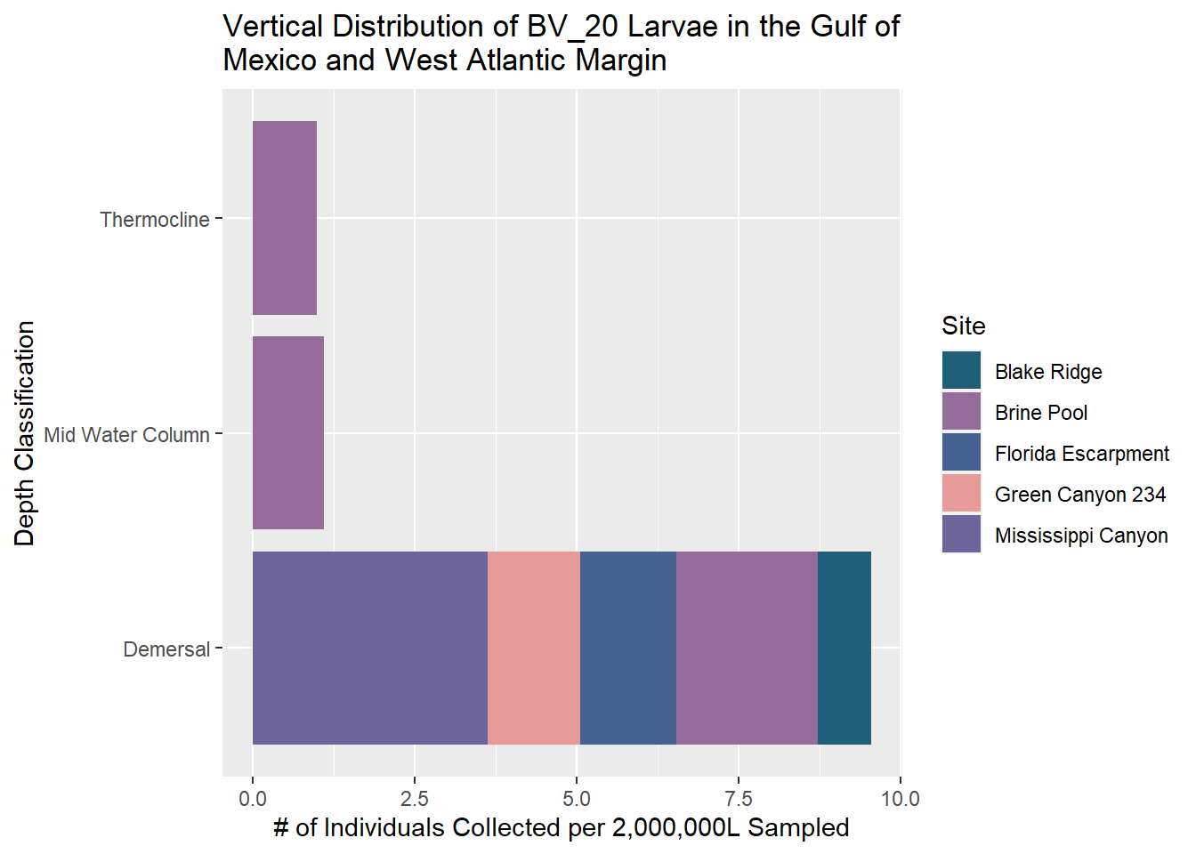
Many BV morphotypes have higher abundance in demersal samples
- BV02, BV03, BV04, BV07-BV12, BV14, BV15, BV20
- BV01 somewhat consistent across depths
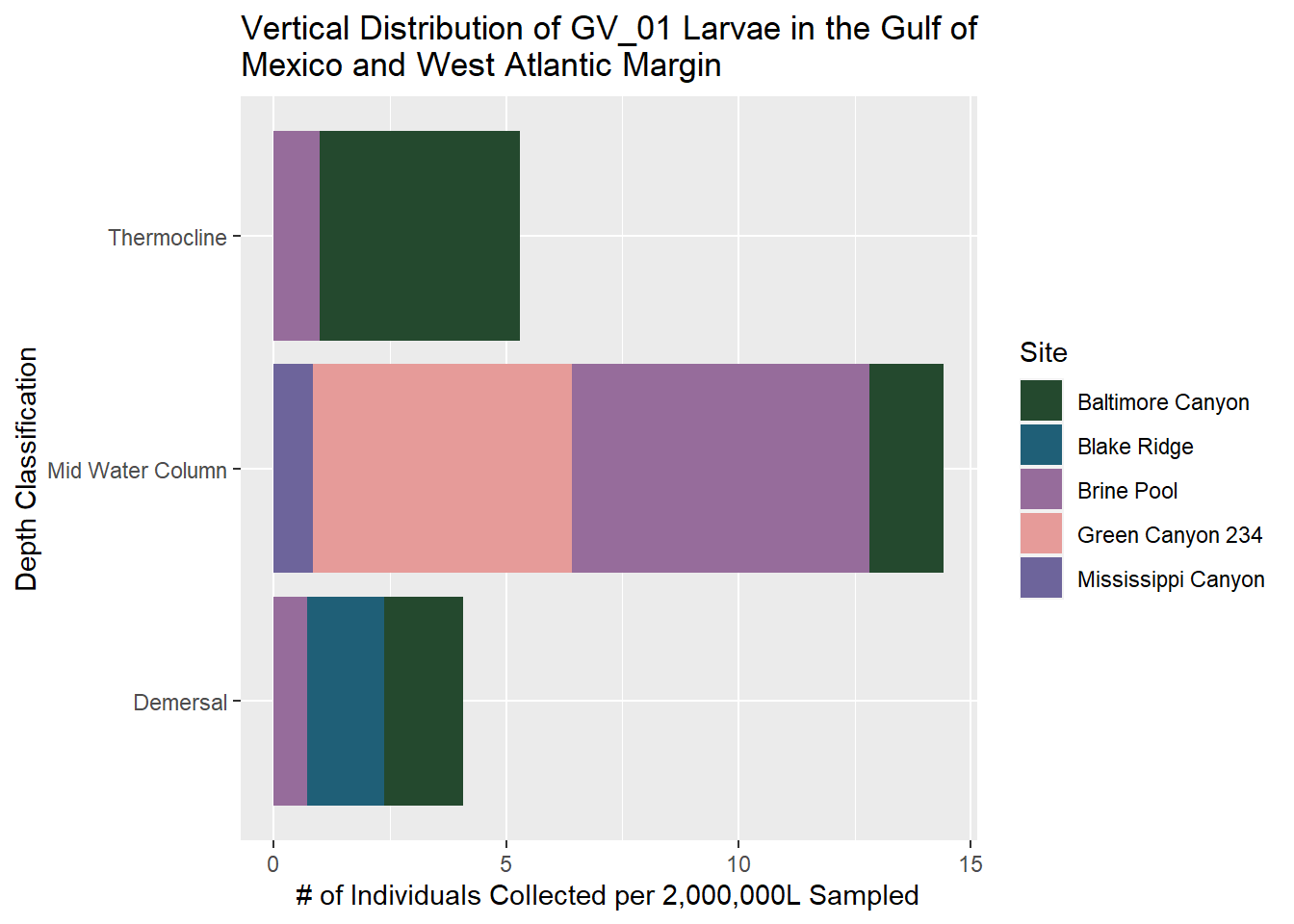
Gv morphotypes vary depth classifications
- Higher Demersal: GV04, GV07, GV16, GV17, GV19, GV20, GV22
- Higher Mid WC: GV09, GV10
- Higher Thermocline: GV02, GV03, GV13, GV14, GV21
- Higher Mid / Thermo: GV01
NE most abundance in Demersal & mid water column.
PC more abundant closer to bottom.
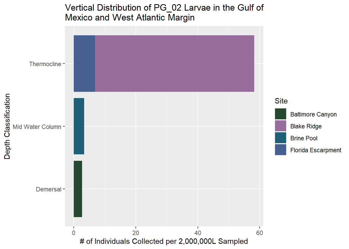
PG more abundance in thermocline (except PG01 similar thermocline and demersal).
PL more abundant higher in water column.
TP most abundant demersally, similar low water column and thermocline.
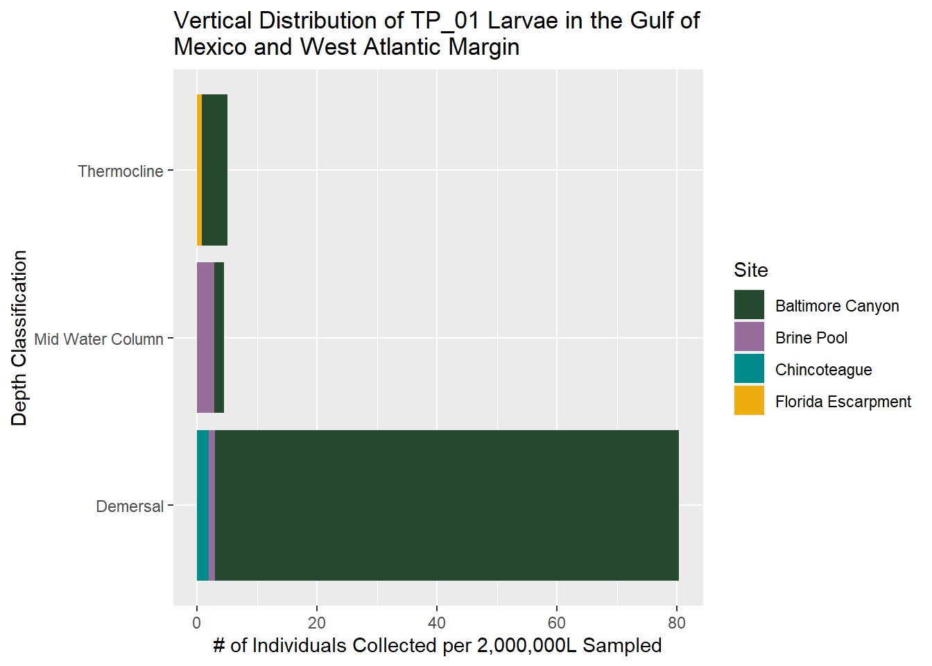
- TP01 more abundant closer to bottom.
ZO slightly more abundant demersal to thermocline

SALT Larval Consensus Summary Statistics

By Dexter Davis - Research Technician for Dr. Shawn Arellano

This Markdown file summarizes the larval data collected with the SyPRID collector on the AUV Sentry during the 2020 EN658 and 2021 TN391 SALT project cruises. This is part of the Seep Animal Larval Transport (SALT) project, NSF Award #1851286.

Data Entry and Subsetting

Summary of Dives from EN658 and TN391

~~~~~~~~~~~~~~~~~~~~~~~~~~~~~~~~~~~~~~~~~~~~~~

Sentry Performance

Summary Tables of Number of Dives

~~~~~~~~~~~~~~~~~~~~~~~~~~~~~~~~~~~~~~~~~~~~~~

Flow Rate Range: 9,261-12,850 Liters/min

Flow Rate Range: 8,674-19,611 Liters/min

Statistics Between Sites and Depth Classifications

~~~~~~~~~~~~~~~~~~~~~~~~~~~~~~~~~~~~~~~~~~~~~~

Sites

Volume Sampled

Larvae Collected

Larval Density

Depth Classifications

Volume Sampled

Larvae Collected

Larval Density

Statistics Within Individual Sites

~~~~~~~~~~~~~~~~~~~~~~~~~~~~~~~~~~~~~~~~~~~~~~

Baltimore Canyon

Volume Sampled

Larvae Collected

Larval Density

Blake Ridge

Volume Sampled

Larvae Collected

Larval Density

Brine Pool

Volume Sampled

Larvae Collected

Larval Density

Bush Hill

Volume Sampled

Larvae Collected

Larval Density

Chincoteague

Volume Sampled

Larvae Collected

Larval Density

Florida Escarpment

Volume Sampled

Larvae Collected

Larval Density

Green Canyon 234

Volume Sampled

Larvae Collected

Larval Density

Mississippi Canyon

Volume Sampled

Larvae Collected

Larval Density

Morphotyping Results

Larval Type Guide

~~~~~~~~~~~~~~~~~~~~~~~~~~~~~~~~~~~~~~~~~~~~~~

Larval Type Presence by Depth

~~~~~~~~~~~~~~~~~~~~~~~~~~~~~~~~~~~~~~~~~~~~~~

Demersal

Mid Water Column

Thermocline

Larval Types Present in Every Depth Classification*:

*Across sites

Community Composition Analysis

~~~~~~~~~~~~~~~~~~~~~~~~~~~~~~~~~~~~~~~~~~~~~~

NMDS Plot

Dendogram

Morphotype Proportion by Depth and Site

~~~~~~~~~~~~~~~~~~~~~~~~~~~~~~~~~~~~~~~~~~~~~~

Significant Morphotypes

All Morphotypes

Brine Pool Seasonality

For Brine Pool, collections from the Fall 2020 EN658 cruise are denoted with the codes Fall, while the other site codes are from the Spring 2021 TN391 cruise.

The color bar along the columns acts as a visual aid for the depth classifications; demersal ( darkblue ), mid water column ( gray-blue ), thermocline ( cyan ).

The vertical line represents the geographical split between the Western Atlantic Margin (left) and the Gulf of Mexico (right) sites or the split between Fall and Spring cruises.

Total Counts for Depth Classifications (Notes)

~~~~~~~~~~~~~~~~~~~~~~~~~~~~~~~~~~~~~~~~~~~~~~

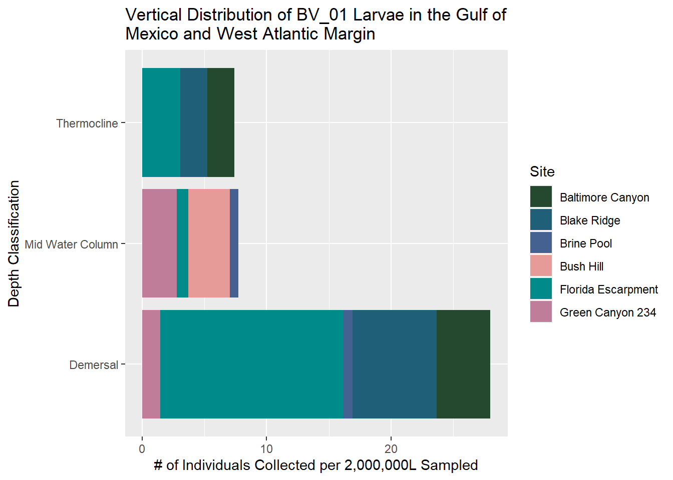
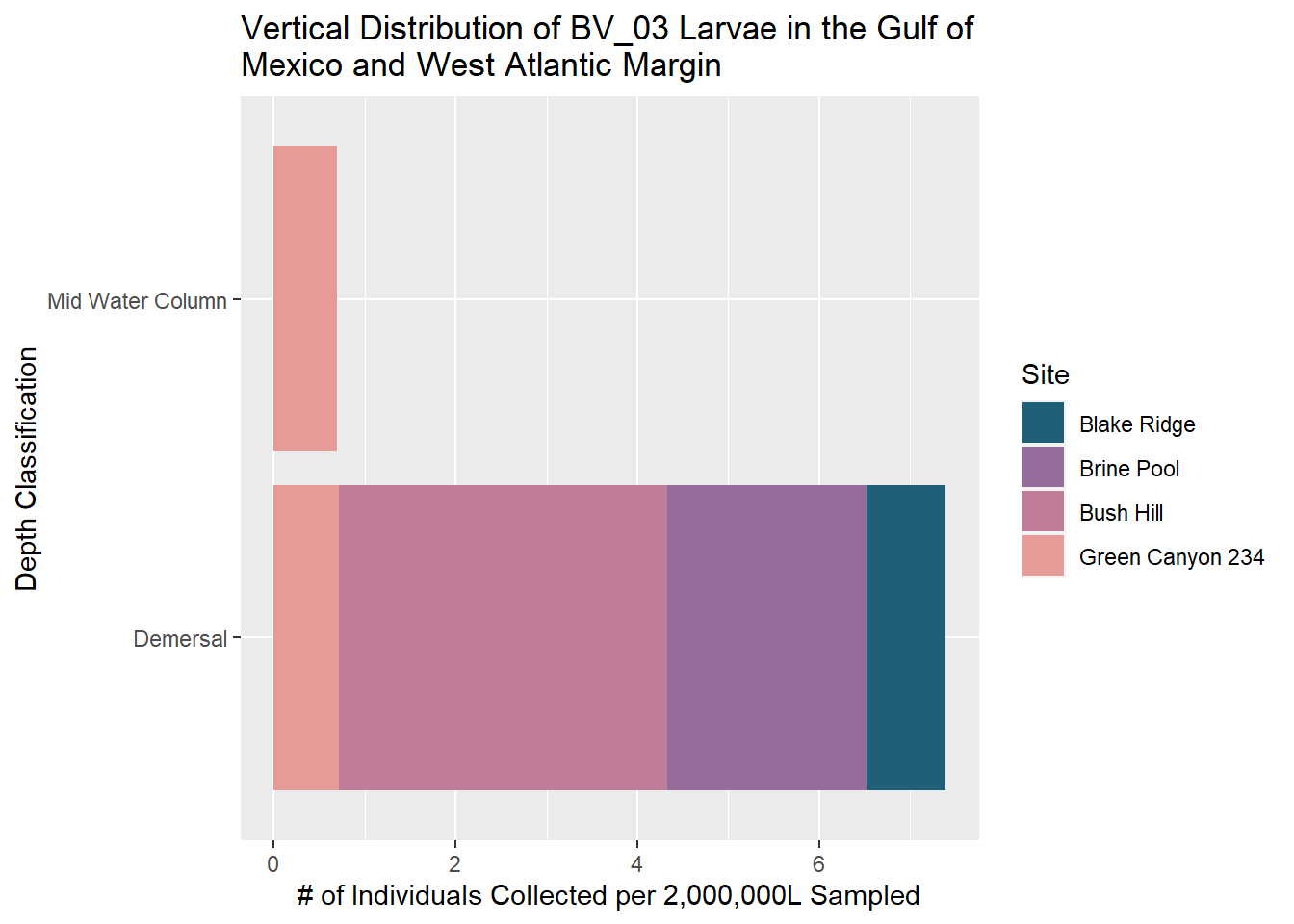
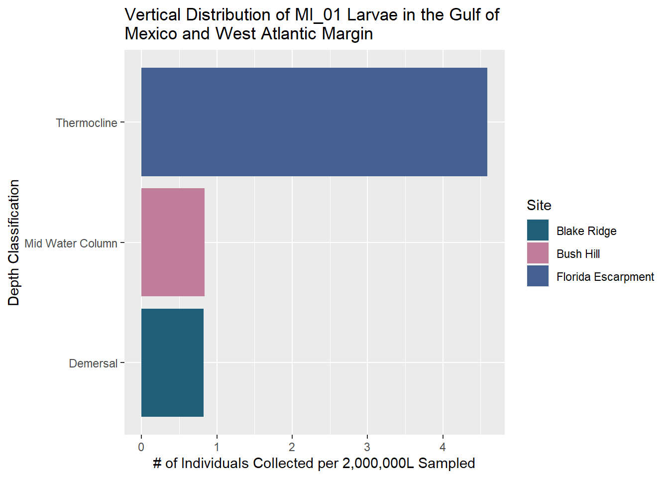
Vertical Distributions of Target Larvae